MANOVA
MANOVA. Dig it!. Comparison to the Univariate. Analysis of Variance allows for the investigation of the effects of a categorical variable on a continuous IV We can also look at multiple IVs, their interaction, and control for the effects of exogenous factors (Ancova)


MANOVA
E N D
Presentation Transcript
MANOVA Dig it!
Comparison to the Univariate • Analysis of Variance allows for the investigation of the effects of a categorical variable on a continuous IV • We can also look at multiple IVs, their interaction, and control for the effects of exogenous factors (Ancova) • Just as Anova and Ancova are special cases of regression, Manova and Mancova are special cases of canonical correlation
Multivariate Analysis of Variance • Is an extension of ANOVA in which main effects and interactions are assessed on a linear combination of DVs • MANOVA tests whether there are statistically significant mean differences among groups on a combination of DVs
MANOVA Example: Examine differences between 2+ groups on linear combinations (V1-V4) of DVs V1 Pros V2 Cons STAGE (5 Groups V3 ConSeff V4 PsySx
MANOVA • A new DV is created that is a linear combination of the individual DVs that maximizes the difference between groups. • In factorial designs a different linear combination of the DVs is created for each main effect and interaction that maximizes the group difference separately. • Also when the IVs have more than two levels the DVs can be recombined to maximize paired comparisons
MANCOVA • The multivariate extension of ANCOVA where the linear combination of DVs is adjusted for one or more continuous covariates. • A covariate is a variable that is related to the DV, which you can’t manipulate, but you want to remove its (their) relationship from the DV before assessing differences on the IVs.
Basic requirements • 2 or more continuous DVs • 1 or more categorical IVs • MANCOVA you also need 1 or more continuous covariates
Anova vs. Manova • Why not multiple Anovas? • Anovas run separately cannot take into account the pattern of covariation among the dependent measures • It may be possible that multiple Anovas may show no differences while the Manova brings them out • MANOVA is sensitive not only to mean differences but also to the direction and size of correlations among the dependents
Anova vs. Manova • Consider the following 2 group and 3 group scenarios, regarding two DVs Y1 and Y2 • If we just look at the marginal distributions of the groups on each separate DV, the overlap suggests a statistically significant difference would be hard to come by for either DV • However, considering the joint distributions of scores on Y1 and Y2 together (ellipses), we may see differences otherwise undetectable
Anova vs. Manova • Now we can look for the greatest possible effect along some linear combination of Y1 and Y2 • The linear combination of the DVs created makes the differences among group means on this new dimension look as large as possible
Anova vs. Manova • So, by measuring multiple DVs you increase your chances for finding a group difference • In this sense, in many cases such a test has more power than the univariate procedure, but this is not necessarily true as some seem to believe • Also conducting multiple ANOVAs increases the chance for type 1 error and MANOVA can in some cases help control for the inflation
Kinds of research questions • The questions are mostly the same as ANOVA just on the linearly combined DVs instead just one DV • What is the proportion of the composite DV explained by the IVs? • What is the effect size? • Is there a statistical and practical difference among groups on the DVs? • Is there an interaction among multiple IVs? • Does change in the linearly combined DV for one IV depend on the levels of another IV? • For example: Given three types of treatment, does one treatment work better for men and another work better for women?
Kinds of research questions • Which DVs are contributing most to the difference seen on the linear combination of the DVs? • Assessment • Roy-Bargmann stepdown analysis • Discriminant function analysis • At this point it should be mentioned that one should probably not do multiple Anovas to assess DV importance, although this is a very common practice • Why? • Because people do not understand what’s actually being done in a MANOVA, so they can’t interpret it • They think that MANOVA will protect their familywise alpha rate • They think the interpretation would be the same and ANOVA is ‘easier’ • As mentioned, the Manova regards the linear combination of DVs, the individual Anovas do not take into account DV interrelationships • If you are really interested in group differences on the individual DVs, then Manova is not appropriate
Kinds of research questions • Which levels of the IV are significantly different from one another? • If there are significant main effects on IVs with more than two levels than you need to test which levels are different from each other • Post hoc tests • And if there are interactions the interactions need to be taken apart so that the specific causes of the interaction can be uncovered • Simple effects
The MV approach to RM • The test of sphericity in repeated measures ANOVA is often violated • Corrections include: • adjustments of the degrees of freedom (e.g. Huynh-Feldt adjustment) • decomposing the test into multiple paired tests (e.g. trend analysis) or • the multivariate approach: treating the repeated levels as multiple DVs (profile analysis)
Theoretical and practical issues in MANOVA • The interpretation of MANOVA results are always taken in the context of the research design. • Fancy statistics do not make up for poor design • Choice of IVs and DVs takes time and a thorough research of the relevant literature • As with any analysis, theory and hypotheses come first, and these dictate the analysis that will be most appropriate to your situation. • You do not collect a bunch of data and then pick and choose among analyses to ‘see if you can find something’.
Theoretical and practical issues in MANOVA • Choice of DVs also needs to be carefully considered, and very highly correlated DVs weaken the power of the analysis • Highly correlated DVs would result in collinearity issues that we’ve come across before, and it just makes sense not to use redundant information in an analysis • One should look for moderate correlations among the DVs • More power will be had when DVs have stronger negative correlations within each cell • Suggestions are in the .3-.7 range • Choice of the order in which DVs are entered in the stepdown analysis has an impact on interpretation, DVs that are causally (in theory) more important need to be given higher priority
Missing data, unequal samples, number of subjects and power • Missing data needs to be handled in the usual ways • E.g. estimation via EM algorithms for DVs • Possible to even use a classification function from a discriminant analysis to predict group membership • Unequal samples cause non-orthogonality among effects and the total sums of squares is less than all of the effects and error added up. This is handled by using either: • Type 3 sums of squares • Assumes the data was intended to be equal and the lack of balance does not reflect anything meaningful • Type 1 sums of square which weights the samples by size and emphasizes the difference in samples is meaningful • The option is available in the SPSS menu by clicking on Model
Missing data, unequal samples, number of subjects and power • You need more cases than DVs in every cell of the design and this can become difficult when the design becomes complex • If there are more DVs than cases in any cell the cell will become singular and cannot be inverted. If there are only a few cases more than DVs the assumption of equality of covariance matrices is likely to be rejected. • Plus, with a small cases/DV ratio power is likely to be very small and the chance of finding a significant effect, even when there is one, is very unlikely • Some programs are available to purchase that can calculate power for multivariate analysis (e.g. PASS) • You can download a SAS macro here • http://www.math.yorku.ca/SCS/sasmac/mpower.html
A word about power • While some applied researchers incorrectly believe that MANOVA would always be more powerful than a univariate approach, the power of a Manova actually depends on the nature of the DV correlations • (1) power increases as correlations between dependent variables with large consistent effect sizes (that are in the same direction) move from near 1.0 toward -1.0 • (2) power increases as correlations become more positive or more negative between dependent variables that have very different effect sizes (i.e., one large and one negligible) • (3) power increases as correlations between dependent variables with negligible effect sizes shift from positive to negative (assuming that there are dependent variables with large effect sizes still in the design). Cole, Maxwell, Arvey 1994
Multivariate normality • Assumes that the DVs, and all linear combinations of the DVs are normally distributed within each cell • As usual, with larger samples the central limit theorem suggests normality for the sampling distributions of the means will be approximated • If you have smaller unbalanced designs than the assumption is assessed on the basis of researcher judgment. • The procedures are robust to type I error for the most part if normality is violated, but power will most likely take a hit • Nonparametric methods are also available
Testing Multivariate Normality • R package (Shapiro-Wilk’s/Royston’s H multivariate normality test in R here) • library(mvnormtest) • mshapiro.test(t(Dataset)) Or • SAS macro (Mardia’s test) • http://support.sas.com/ctx/samples/index.jsp?sid=480 • However, close examination of univariate situation may at least inform if you you’ve got a problem
Outliers • As usual outlier analysis should be conducted • To be assessed in every cell of the design • Transformations are available, deletion might be viable if only a relative very few • Robust Manova procedures are out there but not widely available.
Linearity • MANOVA assume linear relationships among all the DVs • MANCOVA assume linear relationships between all covariate pairs and all DV/covariate pairs • Departure from linearity reduces power as the linear combinations of DVs do not maximize the difference between groups for the IVs
Homogeneity of regression (MANCOVA) • When dealing with covariates it is assumed that there is no IV by covariate interaction • One can include the interaction in the model, and if not statistically significant, rerun without • If there is an interaction, (M)ancova is not appropriate • Implies a different adjustment is needed for each group • Contrast this with a moderator situation in multiple regression with categorical (dummy coded) and continuous variables • In that case we are actually looking for a IV/Covariate interaction
Reliability • As with all methods, reliability of continuous variables is assumed • In the stepdown procedure, in order for proper interpretation of the DVs as covariates the DVs should also have reliability in excess of .8*
Multicollinearity/Singularity • We look for possible collinearity effects in each cell of the design. • Again, you do not want redundant DVs or Covariates
Homogeneity of Covariance Matrices • This is the multivariate equivalent of homogeneity of variance* • Assumes that the variance/covariance matrix in each cell of the design is sampled from the same population so they can be reasonably pooled together to create an error term • Basically the HoV has to hold for the groups on all DVs and the correlation between any two DVs must be equal across groups • If sample sizes are equal, MANOVA has been shown to be robust (in terms of type I error) to violations even with a significant Box’s M test • It is a very sensitive test as is and is recommended by many not to be used
Homogeneity of Covariance Matrices • If sample sizes are unequal then one could evaluate Box’s M test at more stringent alpha. If significant, a violation has probably occurred and the robustness of the test is questionable • If cells with larger samples have larger variances than the test is most likely robustto type I error • though at a loss of power (i.e. type II error increased) • If the cells with fewer cases have larger variances than only null hypotheses are retained with confidence but to reject them is questionable. • i.e. type I error goes up • Use of a more stringent criterion (e.g. Pillai’s criteria instead of Wilk’s)
Different Multivariate test criteria • Hotelling’s Trace • Wilk’s Lambda, • Pillai’s Trace • Roy’s Largest Root • What’s going on here? Which to use?
The Multivariate Test of Significance • Thinking in terms of an F statistic, how is the typical F calculated in an Anova calculated? • As a ratio of B/W (actually mean b/t sums of squares and within sums of squares) • Doing so with matrices involves calculating* BW-1 • We take the between subjects matrix and post multiply by the inverted error matrix
Example Psy Program Silliness Pranksterism 1 8 60 1 7 57 1 13 65 1 15 63 1 12 60 2 15 62 2 16 66 2 11 61 2 12 63 2 16 68 3 17 52 3 20 59 3 23 59 3 19 58 3 21 62 • Dataset example • 1: Experimental • 2: Counseling • 3: Clinical
Example B matrix • To find the inverse of a matrix one must find the matrix such that A-1A = I where I is the identity matrix • 1s on the diagonal, 0s on the off diagonal • For a two by two matrix it’s not too bad W matrix
Example • We find the inverse by first finding the determinate of the original matrix and multiply its inverse by the ‘adjoint’ of that matrix of interest* • Our determinate here is 4688 and so our result for W-1 is You might for practice verify that multiplying this matrix by W will result in a matrix of 1s on the diagonal and zeros off-diagonal
Example • With this new matrix BW-1, we could find the eigenvalues and eigenvectors associated with it.* • For more detail and a different understanding of what we’re doing, click the icon; for some the detail helps. • For the more practically minded just see the R code below • The eigenvalues of BW-1 are (rounded): • 10.179 and 0.226
Let’s get on with it already! • So? • Let’s examine the SPSS output for that data • Analyze/GLM/Multivariate
Wilks’ and Roy’s • We’ll start with Wilks’ lamda • It is calculated as we presented before |W|/|T| = .0729 • It actually is the product of the inverse of the eignvalues+1 • (1/11.179)*(1/1.226) =.073 • Next, take a gander at the value of Roy’s largest root • It is the largest eigenvalue of the BW-1 matrix • The word root or characteristic root is often used for the word eigenvalue
Pillai’s and Hotelling’s • Pillai’s trace is actually the total of our eigenvalues for the BT-1matrix* • Essentially the sum of the variance accounted in the variates • Here we see it is the sum of the eigenvalue/1+eigenvalue ratios • 10.179/11.179 + .226/1.226 = 1.095 • Now look at Hotelling’s Trace • It is simply the sum of the eigenvalues of our • 10.179 + .226 = 10.405
Statistical Significance • Comparing the approximate F for Wilks and Pillai • Wilks is calculated as discussed with canonical correlation • For Pillai’s it is
Statistical Significance • Hotelling-Lawley Trace and Roy’s Largest Root* from SPSS: • s is the number of eigenvalues of the BW-1 matrix (smaller of k-1 vs. p number of DVs) • Again, think of cancorr • Note that s is the number of eigenvalues involved, but for Roy’s greatest root there is only 1 (the largest)
Different Multivariate test criteria • When there are only two levels for an effect that s = 1 and all of the tests will be identical • When there are more than two levels the tests should be close but may not all be similarly sig or not sig
Different Multivariate test criteria • As we saw, when there are more than two levels there are multiple ways in which the data can be combined to separate the groups • Wilk’s Lambda, Hotelling’s Trace and Pillai’s trace all pool the variance from all the dimensions to create the test statistic. • Roy’s largest root only uses the variance from the dimension that separates the groups most (the largest “root” or difference).
Which do you choose? • Wilks’ lambda is the traditional choice, and most widely used • Wilks’, Hotelling’s, and Pillai’s have shown to be robust (type I sense) to problems with assumptions (e.g. violation of homogeneity of covariances), Pillai’s more so, but it is also the most conservative usually. • Roy’s is the more liberal test usually (though none are always most powerful), but it loses its strength when the differences lie along more than one dimension • Some packages will even not provide statistics associated with it • However in practice differences are often seen mostly along one dimension, and Roy’s is usually more powerful in that case (if HoCov assumption is met)
Guidelines from Harlow • Generally Wilks • The others: • Roy’s Greatest Characteristic Root: • Uses only largest eigenvalue (of 1st linear combination) • Perhaps best with strongly correlated DVs • Hotelling-Lawley Trace • Perhaps best with not so correlated DVs • Pillai’s Trace: • Most robust to violations of assumption
Multivariate Effect Size* • While we will have some form of eta-squared measure, typically when comparing groups we like a standardized mean difference • Cohen’s d • Mahalanobis Generalized Distance • Multivariate counterpart • Expresses in a squared metric the distance between the group centroids (the vectors of univariate means) • d is the row/column vector of Cohen’s d for the individual outcome variables, R is the pooled within-groups correlation matrix • Click the smiley for some more technical detail
Post-hoc analysis • If the multivariate test chosen is significant, you’ll want to continue your analysis to discern the nature of the differences. • A first step would be to check the plots of mean group differences for each DV • Graphical display will enhance interpretability and understanding of what might be going on, however it is still in ‘univariate’ mode
Post-hoc analysis • Many run and report multiple univariate F-tests (one per DV) in order to see on which DVs there are group differences; this essentially assumes uncorrelated DVs. • For many this is the end goal, and they assume that running the Manova controls for type I error among the individual tests • Known as the ‘protected F’ • It doesn’t except when: • The null hypothesis is completely true • Which no one ever does follow-ups for • The alternative hypothesis is completely true • In which case there is no possibility for a type I error • The null is true for only one outcome • In short if your goal is to maintain type I error for multiple uni Anovas, then just do a Bonferonni/FDR type correction for them
Post-hoc analysis • Furthemore if the DVs are correlated (as would be the reason for doing a Manova) then individual F-tests do not pick up on this, hence their utility of considering the set of DVs as a whole is problematic • If for example two tests were significant, one would be interpreting them as though the groups were different on separate and distinct measures, which may not be the case
Multiple pairwise contrasts • In a one-way setting one might instead consider performing the pairwise multivariate contrasts, i.e. 2 group MANOVAs • Hotelling’s T2 • Doing so allows for the detail of individual comparisons that we usually want • However type I error is a concern with multiple comparisons, so some correction would still be needed • E.g. Bonferroni, False Discovery Rate
Multiple pairwise contrasts • Example* • Counseling vs. Clinical • Sig • Experimental vs. Clinical • sig • Experimental vs. Counseling • Nonsig • So it seems the clinical folk are standing apart in terms of silliness in chicanery • How so?