Dynamics of DPLL algorithm
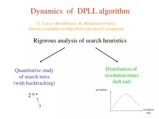
Dynamics of DPLL algorithm. S. Cocco (Strasbourg), R. Monasson (Paris) Articles available on http://www.lpt.ens.fr/~monasson. Rigorous analysis of search heuristics. Distribution of resolution times (left tail). Quantitative study of search trees (with backtracking). probability.

Dynamics of DPLL algorithm
E N D
Presentation Transcript
Dynamics of DPLL algorithm S. Cocco (Strasbourg), R. Monasson (Paris) Articles available on http://www.lpt.ens.fr/~monasson Rigorous analysis of search heuristics Distribution of resolution times (left tail) Quantitative study of search trees (with backtracking) probability 2 N ? resolution time
Analysis of the GUC heuristic p, Chao, Franco ‘90 Frieze, Suen ‘96 t p’,’ (ODE) (unsat) sat
Complete search trees ( > 4.3) DPLL induces a non Markovian evolution of the search tree Imaginary, and parallel building up of the search tree one branch: p(t) , (t) many branches: (p,,t) ODE PDE
Analysis of the search tree growth (I) Average number of branches with clause populations C1, C2, C3 Branching matrix • B(C1, C2, C3;T) exp[ N (c2, c3;t) ] where ci = Ci/N , t = T/N • Distribution of C1 becomes stationary over O(1) time scale
Analysis of the search tree growth (II) t+dt t (PDE) + moving frontier between alive and dead branches
Analysis of the search tree growth (III) t = 0.01 Halt line (Delocalization transition in C1 space) t = 0.05 unsat (sat) t = 0.09
Comparison to numerical experiments unsat sat (nodes) (leaves) Beame, Karp, Pitassi, Saks ‘98
The polynomial/exponentiel crossover sat (exp) unsat (exp) sat (poly) G “dynamical” transition (depends on the heuristic) sat unsat Vardi et al. ’00 Cocco, R.M. ‘01 Achlioptas, Beame, Molloy ‘02 Satisfiable, hard instances 3.003< < 4.3
Fluctuations of complexity for finite instance size Histograms of solving times a=3.5 Exponential regime Complexity = 2 0.035 N Linear regime Very rare! frequence = 2-0.011 N
Application to Stop & Restart resolution Resolution through systematic stop-and-restart of the search: - stop algorithm after time N; - restart until a solution is found. Cocco, R.M. ‘02 Time of resolution : 2 0.035 N 2 0.011 N Halt line for first branch = accumulation of unitary clauses Contradictory region Easy resolution trajectories manage to survive in the contradictory region!
Analysis of the probability of survival (I) Probability of survival of the first branch with clause populations C1, C2, C3 Transition matrix *(1-C1/2/(N-T))C1-1 • B(C1, C2, C3;T) exp[ - N (c1, c2, c3;t) ] where ci = Ci/N , t = T/N • two cases: C1=O(1) (safe regime), C1=O(N) (dangerous regime).
Analysis of the probability of survival (II) • Safe regime: • c1= 0 = log(probability)/N = 0 t t+dt (PDE) • Dangerous regime: c1=O(1) , < 0