Download
1 / 41
410 likes | 578 Vues
Constructing and assessing ocean frontal indexes from satellite SST observations. Mounir Lekouara ( ESA + National Oceanography Centre, Southampton, UK) Supervisors: Pr. Ian Robinson ( National Oceanography Centre, Southampton, UK)

E N D
Constructing and assessing ocean frontal indexes from satellite SST observations Mounir Lekouara ( ESA + National Oceanography Centre, Southampton, UK) Supervisors: Pr. Ian Robinson ( National Oceanography Centre, Southampton, UK) • Christine Gommenginger (National Oceanography Centre, Southampton, UK) Marc Bouvet (European Space Agency)
Outlines • Introduction • Objectives • Front detection techniques • SST datasets for front detection • Frontal indexes • Long term frontal variability
Rational for small scales exploration • Most studies on Earth climate involve spatial and temporal averaging. • Recent dynamical results showed that : • Mesoscale (10-100 km) and submesoscale (1-10 km) have a significant integrated impact on ocean’s primary production budget and on carbon fluxes between the atmosphere and ocean. • A substantial proportion of upwelling, subduction, stratification and lateral stirring in the upper-ocean ocean occur at the small scales. • Satellite sensors resolve fine details of SST which carry the signature of a wide range of underlying dynamical processes. • Study first objective: to explore spatial and temporal variability of small scale transient processes resolved by the SST products.
Ocean surface Fronts • Defined as regions of enhanced horizontal density gradient. • At the sub-mesoscale, the Rossby and Richardson numbers become O(1) in localized regions, leading to an intense ageostrophic circulation and large vertical velocities. • High-resolution dynamical models (1-2 km) show the generation of strong vertical velocities in frontal regions of up to 100m/day (Levy, 2001). • The theory of frontogenesis for cross-front density gradient intensification:1- initiation by mesoscale straining2- disruption of the geostrophic balance for the alongfront flow3- generation of an ageostrophic secondary circulation in the cross-front plane. Adapted from Capet et al. (2008) and Lapeyre et al. (2006)
Unanswered questions Klein et al. (2009) • The short-term/submesoscaledynamics are believed to have a significant impact on the carbon pump, and need to be better understood. • How does the energy cascades from the large and mesoscale (2-D, hydrostatic, geostrophic) to the small scale at which it can be dissipated through 3-D processes ? • What is the role of the fronts in term of mixing and their effect on the carbon cycle ? • Present day Global Circulation Models do not resolve sub-mesocales. Hence there is a need for the parametrization of these processes, in order to improve climate predictions.
Scope of the research • Develop, test and validate front detection algorithms suitable for the new multi-sensor SST products. • Rate the algorithms for frontal detection. • Quantify the ability of Level-4 SST products to resolve small scale features. • Access oceanographic dynamical parameters from observation of the surface SST field, based on: • Results of theoretical research on fronts by others • Additional parameters such as altimetry, and in-situ climatologies of salinity and MLD. • Conception of observational dynamical indices (consistent in space and time) derived from the SST field in this synergetic context. • Focus is on frontogenesis mechanisms and their theoretical effects in term of vertical mixing and restratification.
Satellite-based front detection techniques • Different methodologies to detect the fronts: • Histogram algorithms : “Cayula algorithm”Cayula, J.-F., and P. C. Cornillon (1992), Edge detection algorithm for sst images, Journal of Atmospheric and Oceanic Technology, 9, 67–80. • Simple methods using local statistics of the SST field: gradient, variance, skewness : “Canny algorithm”Canny, J. (1986), A computational approach to edge-detection, Ieee Transactions On Pattern Analysis and Machine Intel ligence, 8, 679–698.
Cayulaalgorithm (1/5) : window decomposition The image is decomposed into 32x32 pixels windows (1.6° x 1.6°)
Cayulaalgorithm (2/5) : • segmentation test of one of the windows
Cayulaalgorithm (4/5) : local level processing to link the limit pixels
Cayula algorithm (5/5) : overview • PARAMETERS • initial resolution of the SST scene • size of the windows in pixels in the segmentation • minimum temperature difference for the histogram analysis to succeed • minimum length for a front to be kept • STRENGTHS • able to deal with missing data (cloud contamination) • deals with fine features, even in presence of noise and without any smoothing • works close to the coastline • returns the “front strength” either with the gradient on the front or with the temperature difference of the two populations of pixels at the window level (more robust to noise). • WEAKNESSES • need of local rectification on a sinusoidal grid • There are many arbitrary parameters. This makes the algorithm look like a “black box” and prevents a simple definition of the detected fronts independent from the algorithm. • It detects several times the strong fronts because of the window segmentation. • It is more complex to implement and more demanding in terms of computational power.
Canny algorithm (1/3) • Local maxima of SST gradient in the gradient direction (crests of gradient magnitude) • Frontal structure reconstruction from raster image.
Canny algorithm (3/3) : overview • PARAMETERS • The initial smoothing filter to minimize noise-induced fronts. • The thresholds T1 and T2. • An optional minimum front length. • WEAKNESSES • It requires an initial smoothing of the data, so it does not resolve the finest features. • It suffers from cloud contamination and does not work close to the coast line. • STRENGTHS • Good for localizing the strong fronts of all scales that are only detected once. • The definition of the fronts that are detected is natural.
Satellite-based front detection techniques • Objective and automatic techniques. • Need for characterizing their performances to retrieve physical parameters. • Challenge: to detect fronts of various scales and intensities that are embedded in a complex turbulent flow, from images that suffer from noise. • Synthetic fronts simulated from SST gradient, temperature step and noise.
Satellite-based front detection techniques • Relative detected front length FL_detected/FL_actual: Cayula Canny σnoise=0.1K σnoise=0K σnoise=0.1K σnoise=0K σnoise=0.2K σnoise=0.3K σnoise=0.2K σnoise=0.3K
Satellite-based front detection techniques • Relative detected front length FL_detected/FL_actualas a function of front orientation Cayula Canny
SST datasets for front detection • “ideal” SST dataset for our study: • Not so much about absolute accuracy, rather the ability to resolve gradients of all scales. • Low level of noise to allow detection of weak fronts. • Maximal spatial/temporal resolution and coverage. • Reflects the temperature of the mixed layer more so than that of atmosphere. • Multi-sensors SST product are the way : • Optimized synoptic coverage, with multi-sensor bias correction which removes patchiness.
SST datasets for front detection • “ideal” SST dataset for our study: • Not so much about absolute accuracy, rather the ability to resolve gradients of all scales. • Low level of noise to allow detection of weak fronts. • Maximal spatial/temporal resolution and coverage. • Reflects the temperature of the mixed layer more so than that of atmosphere. • Multi-sensors SST product are the way : • Optimized synoptic coverage, with multi-sensor bias correction which removes patchiness. Robinson et al. (2012)
SST datasets for front detection • “ideal” SST dataset for our study: • Not so much about absolute accuracy, rather the ability to resolve gradients of all scales. • Low level of noise to allow detection of weak fronts. • Maximal spatial/temporal resolution and coverage. • Reflects the temperature of the mixed layer more so than that of atmosphere. • Multi-sensors SST product are the way : • Optimized synoptic coverage, with multi-sensor bias correction which removes patchiness. • SSTfnd
Limitations of Level-4 SST datasets for front detection • Complementary use of relative qualities of single-sensor data (coverage vs resolution) • But the SST field is smoothed and the resolved scales vary in space within the same Level-4 product • Spatial smoothing introduced to minimize high temporal frequency variations from non-synergetic measurements spatially inconsistent. • Assumption on the correlation length scale that bounds the feature resolution in a non-uniform way.
Limitations of Level-4 SST datasets for front detection ODYSSEA spatial correlation length scale. Autret and Piolle (2007) OSTIA background error standard deviation for 10 km (left) and 100 km (right) synoptic scale features. Donlon et al. (2012).
Limitations of Level-4 SST datasets for front detection • Radial correlation length scale comparison for OSTIA/ODYSSEA/REMSS_MW on 01/01/2008
Limitations of Level-4 SST datasets for front detection • The resolved scales vary in time and space within the same Level-4 product • Due to changes in the available datasets (mission termination or new instrument in orbit). • Due to swath coverage over a day and variable cloud coverage (see Reynolds and Chelton, 2010).
Limitations of Level-4 SST datasets for front detection • Gradient comparison for OSTIA/ODYSSEA/REMSS_MW on January 2008
Limitations of Level-4 SST datasets for front detection • Gradient comparison for OSTIA/ODYSSEA/REMSS_MW on January 2008 after various smoothing (running gaussian)
Level-3 SST datasets for front detection • Level-3 multi-sensor products are ideal for this application: • No smoothing involved • Source sensor is provided, therefore the MW measurements can be discarded in order to ensure spatial and temporal stability of the feature resolution (against cloud coverage). • Unfortunately only 2 years are available to users. Autret and Piolle (2007)
Frontal indices • Matlab routines for fronts detection on SST images and frontal indices construction. • Automatic, parallelized, robust for dealing with a large number of files, parameters and operations. • Density gradient calculation from SST gradient with SSS climatology and equation of state, while assuming a constant salinity across the front (no T/S compensation). • Frontal Index values relying on MLD deeper than 75 m are flagged for potential T/S compensation. Following Rudnick and Martin (2002).
Frontal indices: gradient scaling • SST gradient is scaled to compensate for the product feature resolution following Fox-Kemper et al. (2010). • Assumption: the SST is locally k-2 • The average , over a scale is approximately independent of , where • is the depth-average of the horizontal buoyancy gradient over the mixed layer. • is the SST product feature resolution after smoothing. • is an estimate of the typical local width of fronts. • Assumption: at the surface. • Therefore
Frontal indices: main parameters • The SST dataset • is the size of the running mean filter applied to the density image before the fronts are detected. • is an estimate of the typical local width of mixed layer fronts. • is an estimate of the feature resolution of a SST product after the smoothing stage which depends on the spatial sampling (resolution), the size of the autocorrelation filter applied in the optimal interpolation stage for Level-4 products and the smoothing applied on the image before the fronts are detected. • The Canny thresholds taken equal
Frontal indices: main parameters • The SST dataset • is the size of the running mean filter applied to the density image before the fronts are detected. • is an estimate of the typical local width of mixed layer fronts. • is an estimate of the feature resolution of a SST product after the smoothing stage which depends on the spatial sampling (resolution), the size of the autocorrelation filter applied in the optimal interpolation stage for Level-4 products and the smoothing applied on the image before the fronts are detected. • The Canny thresholds taken equal
Frontal indices: basic indices • Definition of the Frontal Length Index: total length of detected fronts • Definition of the Frontal Gradient Index : • First order measure of stirring and mixing processes • Calculated on high-resolution SST images and integrated over space and/or time. • FLI and FGI allow exploration/diagnostic of scales present in SST datasets.
Frontal indices: basic indices • Definition of the Frontal Length Index: total length of detected fronts • Definition of the Frontal Gradient Index : • First order measure of stirring and mixing processes • Calculated on high-resolution SST images and integrated over space and/or time. • FLI and FGI allow exploration/diagnostic of scales present in SST datasets.
North Atlantic Frontal indices: basic indices FLI ODYSSEA FLI OSTIA Front Length Index (FLI) in Km Km-2day-1 processed on daily ODYSSEA over the North Atlantic region with d=0 Km, Lf=0.5 Km, and ∆s=25 Km. Times when more than 50% of the area MLD is deeper than 75 m are plotted in red. Front Length Index (FLI) in Km Km-2day-1 processed on weekly OSTIA over the North Atlantic region with d=0 Km, Lf=0.5 Km, and ∆s=25 Km. Times when more than 50% of the area MLD is deeper than 75 m are plotted in red. FGI ODYSSEA FGI OSTIA Front Gradient Index (FGI) in Kg m-3 Km-2day-1 processed on daily ODYSSEA over the North Atlantic region with d=0 Km, Lf=0.5 Km, and ∆s=25 Km. Times when more than 50% of the area MLD is deeper than 75 m are plotted in red. Front Gradient Index (FGI) in Kg m-3 Km-2day-1 processed on weekly OSTIA over the North Atlantic region with d=0 Km, Lf=0.5 Km, and ∆s=25 Km. Times when more than 50% of the area MLD is deeper than 75 m are plotted in red.
North Atlantic Frontal indices: basic indices FLI IFREMER_L3_IR FLI REMSS_MW Front Length Index (FLI) in Km Km-2day-1 processed on weekly REMSS_MW over the North Atlantic region with d=0 Km, Lf=0.5 Km, and ∆s=25 Km. Times when more than 50% of the area MLD is deeper than 75 m are plotted in red. Front Length Index (FLI) in Km Km-2day-1 processed on weekly IFREMER_L3_IR over the North Atlantic region with d=0 Km, Lf=0.5 Km, and ∆s=10 Km. Times when more than 50% of the area MLD is deeper than 75 m are plotted in red. FGI REMSS_MW FGI IFREMER_L3_IR • Front Gradient Index (FGI) in Kg m-3 Km-2day-1 processed on daily REMSS_MW over the North Atlantic region with d=0 Km, Lf=0.5 Km, and ∆s=25 Km. Times when more than 50% of the area MLD is deeper than 75 m are plotted in red. Front Gradient Index (FGI) in Kg m-3 Km-2day-1 processed on daily IFREMER_L3_IR over the North Atlantic region with d=0 Km, Lf=0.5 Km, and ∆s=10 Km. Times when more than 50% of the area MLD is deeper than 75 m are plotted in red.
North Atlantic Frontal indices: OSTIA_RAN FGI FGI OSTIA_RAN + OSTIA No smoothing FGI OSTIA_RAN + OSTIA 25 km low-pass filter FGI OSTIA
Frontal indices: OSTIA_RAN FGI FGI OSTIA_RAN No smoothing FGI OSTIA_RAN Climatology fluctuation
Frontal indices: OSTIA_RAN FGI FGI OSTIA_RAN No smoothing Min climatology date Max climatology date
Frontal indices: OSTIA_RAN FGI FGI OSTIA_RAN No smoothing Linear trend
SST data: feedback from a user • My wish-list to Santa: • More Level-3 data! • An measure of the amount of smoothing as a function of time/space in the Level-4 products • No artefact clouds at fronts • Quality indicators not based on the distance from a climatology • In order to allow the detection of signals departing from the mean, even weak ones and at the small scales.