Download
1 / 12
120 likes | 264 Vues
Analytical Approach to Evaporation Problem Using Linearized Richards’ Equation And the application of Green Function. PV/WAVE at UM/MCSR

E N D
Analytical Approach to Evaporation Problem Using Linearized Richards’ Equation And the application of Green Function.
PV/WAVE at UM/MCSR PV-WAVE is a comprehensive package for obtaining solutions for linear and non-linear equations and has a powerful graphics feature that is capable of graphing complex functions. Most if not all the famous mathematical and statistical functions and equations such as Error Function, Gamma Function, FFT, etc, are programmed in pv_wave and are available without much effort. In this article a non-linear equation is graphed using a function from PV-WAVE. This example intends to show users how to invoke and run pv-wave on willow. The pv-wave program listed below shows the strength of pv-wave software. By using only a few instructions pv-wave solves a very complex non-linear equation. The following lines show how to run an example pv-wave job called "chen5_ex.pro" that already exists under "/users/local/appl/examples/pv_wave" on willow. From the willow command prompt, enter:
source /usr/local/vni/wave/bin/wvsetup For tcsh and csh users. /usr/local/vni/wave/bin/wvsetup For ksh and bash userswave Now enter the following command where "chen5_ex.pro" is the name of the pv-wave job: WAVE>.run /users/local/appl/examples/pv_wave/chen5_ex.pro% Compiled module: F. ; % Compiled module: CHEN5_EX. Enter the following to run your job. WAVE> chen5_ex PV-WAVE IMSL Mathematics is initialized. % Compiled module ZEROVECT. When this command appears on the user's terminal, the graph of the function should also appear: The command "chen5_ex" executes the job and draws the graph for the given function. This example graphs and solves equation 13 obtained by J. M. Chen et al. in their paper published in Water Resources Research, Vol. 37, No. 4 pp.1091-1093, April, 2001. The t-axis on the graph represents the time in seconds and f(t) represents the rain fall intensity q(T), the rate at which the rainfall piles up on a certain soil (silt loam).
For more information refer to the above paper by Chen, et al. Results obtained here matches those obtained by Chen and the graph here is his figure 1. This equation was later used by Sam G. of IT to obtain the graph of certain functions needed in solving Richards' Equation. Please call Sam Gordji at 5022, e-mail: ccsam@olemiss.edu if you have questions about pv-wave. **Please note that this example requires X-win to run.** See: http://www.mcsr.olemiss.edu/computing/xwin32.html. Listing for pv-wave program follows: *** This graphs equation 13 on pg. 1092 of Ap. 2001 of WRR paper by J.M. Chen. **** ** For the case when gama=5 & n=0, F(T)=5 ** THE NEXT LINE IS THE START OF THE PROGRAM. This program should be named "chen5_ex.pro".
chen5_ex.pro • ; *** This graphs, eq. 13 on pg. 1092 of Ap. 2001 of WRR paper by J.M. Chen. **** • ; ** This is for the case when gama=5 & n=0, F(T)=5 *** • ; Next 3 lines defines the problem. • FUNCTION f,t • RETURN, .0018455*(SQRT(t/3.14)+1.)*exp(-0.25*t) • END • ; pro or procedure tell the compiler that a user prog. module follows • PRO chen5_ex • ; activate the Math toolkit • MATH_INIT • t= INTERPOL([0,100],400000) • ; plot statement plots f, f(t) with the range of 0 to 2 and .0018 to .0023 • plot, t, f(t), xrange=[0,2], yrange=[.0018,.0023] • ; zero=zerovect(f(t),t) • ; print, zero • ; oplot , plots the second plot in our case it plots over the original plot • oplot, [zero], [f(zero)], psym=6 • END
Program Zerovec_ex.pro Solves Equation 14 or 15 to obtain time for surface saturation • ;;;;;;;;;zerovec_ex.pro, As before the three lines are to define the problem;;;;;;;;;;;;;; • FUNCTION f,t • RETURN, 2.18*SQRT((1/3.14)*t)*exp(-0.25*t) - 0.216 • END • PRO zerovec_ex • ; pro = procedure zerovec_ex • MATH_INIT • ; call Mathematical Tool Kit from IMSL/PV • t= INTERPOL([0,14],10000) • ; Interpolate the above function from 0 to 14 with n=10000 • ; choosing smaller number for n may yield a curve that is not smooth • ; or may yeild bad answers • plot, t, f(t) • ; plot t and f(t) • zero=zerovect(f(t),t) • ; call zerovect and find zeros of the above function • print, zero • ;print the results • oplot, [zero], [f(zero)], psym=6 • xyouts, .2, .5, ' Computed zero is at x=' +STRING(zero(0))+' and x='+STRING(zero(1)) • ; print the answers on the graph as well • END • ;;;;;;;;;;;;;;;;;;;;;;;;;;;;;;;;;;;;;;;;;;;;;;;;;;;;;;;;;;;;;;;;;;;;;;;;;;;; • ;;;;;;;;;
Note that the above equation has 2 solution t=0.03131, 11.914