Quantitative Analysis

1. Quantitative Analysis Lecture 2 Discrete Probability Functions Prepared by Dr. Ikhlaas Gurrib

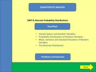
2. Introduction • In the field of quantitative analysis, we often use the term Random Variable. • Random Variable is a quantity resulting from a random experiment that, by chance, can assume different values. Such as, number of defective light bulbs produced during a week. • Also, we said a Discrete Random Variable is a variable which can assume only integer values, such as, 7, 9, and so on. In other words, a discrete random variable cannot take fractions as value. Things such as people, cars, or defectives are things we can count and are discrete items. • 2 types of Random Discrete Prob. Distribution we shall discuss are: • Binomial Distribution • Poisson Distribution

3. Mean, and Variance of Discrete Random Variables • The equation for computing the mean, or expected value of discrete random variables is as follows:Mean = E(X) = Summation[X.P(X)]where: E(X) = expected value, X = an event, and P(X) = probability of the event

5. An example • Suppose a charity organization is mailing printed return-address stickers to over one million homes in the U.S. Each recipient is asked to donate either $1, $2, $5, $10, $15, or $20. Based on past experience, the amount a person donates is believed to follow the following probability distribution:X:..... $1......$2........$5......$10.........$15......$20P(X)....0.1.....0.2.......0.3.......0.2..........0.15.....0.05What is expected that an average donor to contribute, and what is the standard deviation?

6. Solution • 1)......(2).......(3).............(4)..................(5)..........................................(6)X......P(X)....X.P(X).......X - mean......[(X - mean)]squared............... (5)x(2)1.......0.1......0.1...........- 6.25...............39.06........................................3.9062.......0.2......0.4...........- 5.25...............27.56........................................5.5125.......0.3......1.5...........- 2.25.................5.06........................................1.51810.....0.2......2.0.............2.75.................7.56........................................1.51215.....0.15....2.25...........7.75...............60.06........................................9.00920.....0.05....1.0...........12.75.............162.56.........................................8.125 Total...........7.25 = E(X)....................................................................29.585Therefore, the expected value is $7.25, and standard deviation is the square root of $29.585, which is equal to $5.55. In other words, an average donor is expected to donate $7.25 with a standard deviation of $5.55.

7. Binomial Distribution • One of the most widely known of all discrete probability distributions is the binomial distribution. Several characteristics underlie the use of the binomial distribution. Characteristics of the Binomial Distribution: 1. The experiment consists of n identical trials. 2. Each trial has only one of the two possible mutually exclusive outcomes, success or a failure. 3. The probability of each outcome does not change from trial to trial, and 4. The trials are independent, thus we must sample with replacement.

8. An important assumption • Note that if the sample size, n, is less than 5% of the population, the independence assumption is not of great concern. Therefore the acceptable sample size for using the binomial distribution with samples taken without replacement is [n<5%N] where n is equal to the sample size, and N stands for the size of the population. • The birth of children (male or female), true-false or multiple-choice questions (correct or incorrect answers) are some examples of the binomial distribution.

9. Binomial Equation • When using the binomial formula to solve problems, all that is necessary is that we are able to identify three things: • the number of trials (n), • the probability of a success on any one trial(p), and • the number of successes desired (X).

10. Binomial Distribution where: n = the sample size or the number of trials, X = the number of successes desired, p = probability of getting a success in one trial, and q = (1 - p) = the probability of getting a failure in one trial.

11. An Example • Suppose that 4% of all TVs made by W&B Company in 2010 are defective. If eight of these TVs are randomly selected from across the country and tested, what is the probability that exactly three of them are defective? Assume that each TV is made independently of the others.In this problem, n=8, X=3, p=0.04, and q=(1-p)=0.96. Plugging these numbers into the binomial formula, we get: • P(X=3) = 0.00292 or 0.29% • The mean is equal to (n) x (p) = (8)(0.04)=0.32, • The variance is equal to np (1 - p) = (0.32)(0.96) = 0.31, and the standard deviation is 0.6.

12. The Binomial Table • Quantitative Analysts previously used tables containing pre-solved probabilities. • We have now evolved by using Excel which simplify the calculations. • Use BINOMDIST Function.

13. Example 2 • Suppose that an examination consists of six true and false questions, and assume that a student has no knowledge of the subject matter. The probability that the student will guess the correct answer to the first question is 30%. Likewise, the probability of guessing each of the remaining questions correctly is also 30%. What is the probability of getting more than three correct answers?

14. Solution • For the above problem, n = 6, p = 0.30, and X >3. In the above table, search along the row of p values for 0.30. The problem is to locate the P(X > 3). Thus, the answer involves summing the probabilities for X = 4, 5, and 6. • P (X > 3) = Summation of {P (X=4) + P(X=5) +P(X=6)} = (0.060)+(0.010)+(0.001) = 0.071 or 7.1%. Thus, we may conclude that if 30% of the exam questions are answered by guessing, the probability is 0.071 (or 7.1%) that more than four of the questions are answered correctly by the student.

15. A Final note on Binomial Distributions • Graphing the Binomial Distribution • The graph of a binomial distribution can be constructed by using all the possible X values of a distribution and their associated probabilities. The X values are graphed along the X axis, and the probabilities are graphed along the Y axis. • Note that the graph of the binomial distribution has three shapes: If p<0.5, the graph is positively skewed, if p>0.5, the graph is negatively skewed, and if p=0.5, the graph is symmetrical. • The skewness is eliminated as n gets large. In other words, if n remains constant but p becomes larger and larger up to 0.50, the shape of the binomial probability distribution becomes more symmetrical. If p remains the same but n becomes larger and larger, the shape of the binomial probability distribution becomes more symmetrical.

16. The Poisson Distribution • Named after Simeon-Denis Poisson (1781-1840), a French mathematician, the Poisson distribution depends only on the average number of occurrences per unit time of space. • There is no n, and no p. The Poisson probability distribution provides a close approximation to the binomial probability distribution when n is large and p is quite small or quite large. • In other words, if n>20 and np<=5 [or n(1-p)<="5]," then we may use poisson distribution as an approximation to binomial distribution.

17. When do we use it? • The Poisson distribution arises when you count a number of events across time or over an area. You should think about the Poisson distribution for any situation that involves counting events. • Some examples are: - the number of Emergency Department visits by an infant during the first year of life, - the number of incidents of apna and bradycardia in a pre-term infant. • the number of items demanded per customer from an inventory • the number of ‘on time’ arrivals during the Christmas night period. Sometimes, you will see the count represented as a rate, such as the number of deaths per year due to horse kicks, or the number of defects per square yard.

18. Important Assumptions • The Poisson distribution assumes: • no limit on the number of occurrences • that occurrences are independent How to test if the Poisson distribution fits your data? (1) The simplest and handiest way is to see if the variance is roughly equal to the mean for your Poisson data. (2) A histogram of the Poisson data should be skewed right, though the skewness becomes less pronounced as the mean increases.

19. Computation • Probabilities using Poisson distribution can be computed using the Excel function as follows: • POISSON(x,mean,cumulative)

20. An example • Suppose the average number of customers arriving at an ATM during lunch hour is λ=12 customers per hour. • The probability that exactly x customers will arrive during the hour is • P(x) = e-12*12x = 0.00007 x!

21. Graphical Analysis • Like the binomial distribution, the specific shape depends on the parameter λ. The distribution is more skewed for smaller values.

22. Use of Poisson approximations • The Poisson probability distribution provides a close approximation to the binomial probability distribution when: • n is large and p is quite small or quite large. In other words, if n>20 and np<=5 [or nq<=5], then we may use Poisson distribution as an approximation to the Binomial distribution.

23. Review • The Binomial and Poisson distributions are two commonly used discrete probability distribution functions. • Their results are only effective if the assumptions of the models are met.