Download
1 / 74
770 likes | 1.08k Vues
Solar Interior Magnetic Fields and Dynamos. Steve Tobias (Leeds). 5th Potsdam Thinkshop, 2007. Observations. Fields, flows and activity. Large-scale activity. Fields, flows and activity. Observations: Solar. Magnetogram of solar surface shows radial component of the

E N D
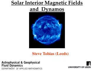
Solar Interior Magnetic Fields and Dynamos Steve Tobias (Leeds) 5th Potsdam Thinkshop, 2007
Observations Fields, flows and activity
Large-scale activity Fields, flows and activity
Observations: Solar Magnetogram of solar surface shows radial component of the Sun’s magnetic field. Active regions: Sunspot pairs and sunspot groups. Strong magnetic fields seen in an equatorial band (within 30o of equator). Rotate with sun differentially. Each individual sunspot lives ~ 1 month. As “cycle progresses” appear closer to the equator.
Sunspots Dark spots on Sun (Galileo) cooler than surroundings ~3700K. Last for several days (large ones for weeks) Sites of strong magnetic field (~3000G) Joy’s Law: Axes of bipolar spots tilted by ~4 deg with respect to equator Hale’s Law: Arise in pairs with opposite polarity Part of the solar cycle Fine structure in sunspot umbra and penumbra SST
Observations Solar (a bit of theory) Sunspot pairs are believed to be formed by the instability of a magnetic field generated deep within the Sun. Flux tube rises and breaks through the solar surface forming active regions. This instability is known as Magnetic Buoyancy- we are just beginning to understand how strong coherent “tubes” may form from weaker layers of field. Kersalé et al (2007)
Observations Solar (a bit of theory) Once structures are formed they rise and break through the solar surface to form active regions – this process is not well understood e.g. why are sunspots so small?
Observations: Solar BUTTERFLY DIAGRAM: last 130 years Migration of dynamo activity from mid-latitudes to equator Polarity of sunspots opposite in each hemisphere (Hale’s polarity law). Tend to arise in “active longitudes” DIPOLAR MAGNETIC FIELD Polarity of magnetic field reverses every 11 years. 22 year magnetic cycle.
Three solar cycles of sunspots Courtesy David Hathaway
Observations Solar • Solar cycle not just visible in sunspots • Solar corona also modified as cycle progresses. • Weak polar magnetic field has mainly one polarity at each pole and two poles have opposite polarities • Polar field reverses every 11 years – but out of phase with the sunspot field (see next slide) • Global Magnetic field reversal.
Observations Solar • Solar cycle not just visible in sunspots • Solar corona also modified as cycle progresses. • Weak polar magnetic field has mainly one polarity at each pole and two poles have opposite polarities • Polar field reverses every 11 years – but out of phase with the sunspot field. • Global Magnetic field reversal.
Observations: Solar SUNSPOT NUMBER: last 400 years Modulation of basic cycle amplitude (some modulation of frequency) Gleissberg Cycle: ~80 year modulation MAUNDER MINIMUM: Very Few Spots , Lasted a few cycles Coincided with little Ice Age on Earth Abraham Hondius (1684)
Observations: Solar RIBES & NESME-RIBES (1994) BUTTERFLY DIAGRAM: as Sun emerged from minimum Sunspots only seen in Southern Hemisphere Asymmetry; Symmetry soon re-established. No Longer Dipolar? Hence: (Anti)-Symmetric modulation when field is STRONG Asymmetric modulation when field is weak
14 C 10 Be Observations: Solar (Proxy) PROXY DATA OF SOLAR MAGNETIC ACTIVITY AVAILABLE SOLAR MAGNETIC FIELD MODULATES AMOUNT OF COSMIC RAYS REACHING EARTH responsible for production of terrestrial isotopes : stored in ice cores after 2 years in atmosphere : stored in tree rings after ~30 yrs in atmosphere BEER (2000)
Observations: Solar (Proxy) Cycle persists through Maunder Minimum (Beer et al 1998) DATA SHOWS RECURRENT GRAND MINIMA WITH A WELL DEFINED PERIOD OF ~ 208 YEARS Distribution of “maxima in activity” is consistent with a Gamma distribution. we have a current maximum – life expectancy for this is short (Abreu et al 2007) Wagner et al (2001)
Solar Structure Solar Interior • Core • Radiative Interior • (Tachocline) • Convection Zone Visible Sun • Photosphere • Chromosphere • Transition Region • Corona • (Solar Wind)
The Large-Scale Solar Dynamo • Helioseismology shows the internal structure of the Sun. • Surface Differential Rotation is maintained throughout the Convection zone • Solid body rotation in the radiative interior • Thin matching zone of shear known as the tachocline at the base of the solar convection zone (just in the stable region).
Torsional Oscillations and Meridional Flows • In addition to mean differential rotation there are other large-scale flows • Torsional Oscillations • Pattern of alternating bands of slower and faster rotation • Period of 11 years (driven by Lorentz force) • Oscillations not confined to the surface (Vorontsov et al 2002) • Vary according to latitude and depth
Torsional Oscillations and Meridional Flows • Meridional Flows • Doppler measurements show typical meridional flows at surface polewards: velocity 10-20ms-1 (Hathaway 1996) • Poleward Flow maintained throughout the top half of the convection zone (Braun & Fan 1998) • Large fluctuations about this mean with often evidence of multiple cells and strong temporal variation with the solar cycle (Roth 2007) • No evidence of returning flow • Meridional flow at surface advects flux towards the poles and is probably responsible for reversing the surface polar flux
Observations: Stellar (Solar-Type Stars) Stellar Magnetic Activity can be inferred by amount of Chromospheric Ca H and K emission Mount Wilson Survey (see e.g. Baliunas ) Solar-Type Stars show a variety of activity. Cyclic, Aperiodic, Modulated, Grand Minima
Observations: Stellar (Solar-Type Stars) • Activity is a function of spectral type/rotation rate of star • As rotation increases: activity increases • modulation increases • Activity measured by the relative Ca II HK flux density • (Noyes et al 1994) • But filling factor of magnetic fields also changes • (Montesinos & Jordan 1993) • Cycle period • Detected in old slowly-rotating G-K stars. • 2 branches (I and A) (Brandenburg et al 1998) • WI ~ 6 WA (including Sun) Wcyc/Wrot ~ Ro-0.5(Saar & Brandenburg 1999)
I (i) Small-scale activity Fields and flows and activity
Basic Dynamo Theory Dynamo theory is the study of the generation of magnetic field by the inductive motions of an electrically conducting plasma. Non-relativistic Maxwell equations + Ohm’s Law + Navier-Stokes equations…
Basic Dynamo Theory Dynamo theory is the study of the generation of magnetic field by the inductive motions of an electrically conducting plasma. Induction Eqn Momentum Eqn Including Rotation, Gravity etc Nonlinear in B A dynamo is a solution of the above system for which B does not decay for large times. Hard to find simple solutions (antidynamo theorems)
Why is dynamo Theory so hard? Why are there no nice analytical solutions? Why don’t we just solve the equations on a computer? Dynamos are sneaky and parameter values are extreme It can be shown that a flow or magnetic field that is “too simple” (i.e. has too much symmetry) cannot lead to or be generated by dynamo action. The most famous example is Cowling’s Theorem. “No Axisymmetric magnetic field can be maintained by a dynamo” Cowling’s Theorem (1934)
Basics for the Sun Dynamics in the solar interior is governed by the following equations of MHD INDUCTION MOMENTUM CONTINUITY ENERGY GAS LAW
1020 1016 1013 1012 1010 106 10-7 10-7 105 1 10-3 10-6 10-4 1 0.1-1 10-3-0.4 BASE OF CZ Basics for the Sun PHOTOSPHERE (Ossendrijver 2003)
Modelling Approaches • Because of the extreme nature of the parameters in the Sun and other stars there is no obvious way to proceed. • Modelling has typically taken one of three forms • Mean Field Models (~85%) • Derive equations for the evolution of the mean magnetic field (and perhaps velocity field) by parametrising the effects of the small scale motions. • The role of the small-scales can be investigated by employing local computational models • Global Computations (~5%) • Solve the relevant equations on a massively-parallel machine. • Either accept that we are at the wrong parameter values or claim that parameters invoked are representative of their turbulent values. • Maybe employ some “sub-grid scale modelling” e.g. alpha models • Low-order models • Try to understand the basic properties of the equations with reference to simpler systems (cf Lorenz equations and weather prediction) • All 3 have strengths and weaknesses
The Geodynamo • The Earth’s magnetic field is also generated by a dynamo located in its outer fluid core. • The Earth’s magnetic field reverses every 106 years on average. • Conditions in the Earth’s core much less turbulent and are approaching conditions that can be simulated on a computer (although rotation rate causes a problem).
Mean-field electrodynamics A basic physical picture W-effect – poloidal toroidal
Mean-field electrodynamics A basic physical picture a-effect – toroidal poloidal poloidal toroidal
Alpha-effect Omega-effect Turbulent diffusivity BASIC PROPERTIES OF THE MEAN FIELD EQUATIONS This can be formalised by separating out the magnetic field into a mean (B0) and fluctuating part (b) and parameterising the small-scale interactions In their simplest form the mean field equation becomes Now consider simplest case where a = a0 cos q andU0 = U0 sin q ef In contrast to the induction equation, this can be solved for axisymmetric mean fields of the form
BASIC PROPERTIES OF THE MEAN FIELD EQUATIONS • In general B0 takes the form of an exponentially growing dynamo wave that propagates. • Direction of propagation depends on sign of dynamo number D. • If D > 0 waves propagate towards the poles, • If D < 0 waves propagate towards the equator. • In this linear regime the frequency of the magnetic cycle Wcyc is proportional to |D|1/2 • Solutions can be either dipolar or quadrupolar
Some solar dynamo scenarios Distributed, Deep-seated, Flux Transport, Interface, Near-Surface. This is simply a matter of choosing plausible profiles for a and b depending on your prejudices or how many of the objections to mean field theory you take seriously!
Distributed Dynamo Scenario • PROS • Scenario is “possible” wherever convection and rotation take place together • CONS • Computations show that it is hard to get a large-scale field • Mean-field theory shows that it is hard to get a large-scale field (catastrophic a-quenching) • Buoyancy removes field before it can get too large
Near-surface Dynamo Scenario • This is essentially a distributed dynamo scenario. • The near-surface radial shear plays a key role. • Magnetic features tend to move with rotation rate at the bottom of the near surface shear layer. • Same pros and cons as before. • Brandenburg (2006)
Flux Transport Scenario • Here the poloidal field is generated at the surface of the Sun via the decay of active regions with a systematic tilt (Babcock-Leighton Scenario) and transported towards the poles by the observed meridional flow • The flux is then transported by a conveyor belt meridional flow to the tachocline where it is sheared into the sunspot toroidal field • No role is envisaged for the turbulent convection in the bulk of the convection zone.
Flux Transport Scenario • PROS • Does not rely on turbulent a-effect therefore all the problems of a-quenching are not a problem • Sunspot field is intimately linked to polar field immediately before. • CONS • Requires strong meridional flow at base of CZ of exactly the right form • Ignores all poloidal flux returned to tachocline via the convection • Effect will probably be swamped by “a-effects” closer to the tachocline • Relies on existence of sunspots for dynamo to work (cf Maunder Minimum)
Modified Flux Transport Scenario • In addition to the poloidal flux generated at the surface, poloidal field is also generated in the tachocline due to an MHD instability. • No role is envisaged for the turbulent convection in the bulk of the convection zone in generating field • Turbulent diffusion still acts throughout the convection zone.
Interface/Deep-Seated Dynamo • The dynamo is thought to work at the interface of the convection zone and the tachocline. • The mean toroidal (sunspot field) is created by the radial diffential rotation and stored in the tachocline. • And the mean poloidal field (coronal field) is created by turbulence (or perhaps by a dynamic a-effect) in the lower reaches of the convection zone
Interface/Deep-Seated Dynamo • PROS • The radial shear provides a natural mechanism for generating a strong toroidal field • The stable stratification enables the field to be stored and stretched to a large value. • As the mean magnetic field is stored away from the convection zone, the a-effect is not suppressed • Separation of large and small-scale magnetic helicity • CONS • Relies on transport of flux to and from tachocline – how is this achieved? • Delicate balance between turbulent transport and fields. • “Painting ourselves into a corner”
Mean-field electrodynamics A basic physical picture W-effect – poloidal toroidal
Mean-field electrodynamics A basic physical picture a-effect – toroidal poloidal poloidal toroidal
Some solar dynamo scenarios Distributed, Deep-seated, Flux Transport, Interface, Near-Surface. This is simply a matter of choosing plausible profiles for a and b depending on your prejudices or how many of the objections to mean field theory you take seriously!
Distributed Dynamo Scenario • PROS • Scenario is “possible” wherever convection and rotation take place together • CONS • Computations show that it is hard to get a large-scale field • Mean-field theory shows that it is hard to get a large-scale field (catastrophic a-quenching) • Buoyancy removes field before it can get too large
Near-surface Dynamo Scenario • This is essentially a distributed dynamo scenario. • The near-surface radial shear plays a key role. • Magnetic features tend to move with rotation rate at the bottom of the near surface shear layer. • Same pros and cons as before. • Brandenburg (2006)
Flux Transport Scenario • Here the poloidal field is generated at the surface of the Sun via the decay of active regions with a systematic tilt (Babcock-Leighton Scenario) and transported towards the poles by the observed meridional flow • The flux is then transported by a conveyor belt meridional flow to the tachocline where it is sheared into the sunspot toroidal field • No role is envisaged for the turbulent convection in the bulk of the convection zone.
Flux Transport Scenario • PROS • Does not rely on turbulent a-effect therefore all the problems of a-quenching are not a problem • Sunspot field is intimately linked to polar field immediately before. • CONS • Requires strong meridional flow at base of CZ of exactly the right form • Ignores all poloidal flux returned to tachocline via the convection • Effect will probably be swamped by “a-effects” closer to the tachocline • Relies on existence of sunspots for dynamo to work (cf Maunder Minimum)
Modified Flux Transport Scenario • In addition to the poloidal flux generated at the surface, poloidal field is also generated in the tachocline due to an MHD instability. • No role is envisaged for the turbulent convection in the bulk of the convection zone in generating field • Turbulent diffusion still acts throughout the convection zone.