Download
1 / 57
590 likes | 732 Vues
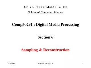
UNIVERSITY of MANCHESTER School of Computer Science Comp30291 : Digital Media Processing Section 6 Sampling & Reconstruction. Introduction. This section concerns the sampling & digitisation of analogue signals.

E N D
UNIVERSITY of MANCHESTER School of Computer Science Comp30291 : Digital Media Processing Section 6 Sampling & Reconstruction Comp30291 Sectn 6
Introduction • This section concerns the sampling & digitisation of analogue signals. • The signals may then be processed digitally and/or transmitted in digital form. • Resulting digital signals often need to be converted back to analogue form or “reconstructed”. • Reconstruction is also considered in this section. Comp30291 Sectn 6
xa(t) |Xa(j)| t An analogue signal & its magnitude spectrum. Comp30291 Sectn 6
x[5] xa(t) x[3] x[2] x[1] X[0] x[-1] -3T -2T t -T T 2T 3T 4T 5T x[-2] x[-3] Sampling an analogue signal Measure xa(t) at intervals T to obtain {x[n]}: { ..., x[-1], x[0], x[1], x[2], x[3], ... } x[1] = xa(T), x[2] = xa(2T), etc. Comp30291 Sectn 6
xa(4T) xS(t) xa(2T) xa(T) x ( - T) a - 3T - 2T t T 2T 3T 4T 5T -T x ( - 2T) a Invent a new signal xS(t) = sampleT{xa(t)} Measure xa(t) at 0, T, 2T, ... & represent by analogue impulses. Comp30291 Sectn 6
Volts As width 0, & height with strength remaining at 1 we get ‘unitimpulse’ More pulses of strength 1 5 Pulse of strength 20.5=1 4 Voltage pulse of strength 11=1 3 1 2 1 t 1 1/8 1/4 1/2 Analogue ‘unit impulse’ Comp30291 Sectn 6
Analogue ‘impulse’ of strength A Volts Even narrower pulse of strength A As width 0, & height with strength remaining at A we get impulse of strength A Narrower pulse of strength 2A0.5=A 5 Voltage pulse of strength 1A=A 4 3 A 2 A 1 t 1 1/4 1/2 Comp30291 Sectn 6
DTFT of {x[n]} It may be shown that: DTFT of {x[n]} = Fourier transform of xS(t) i.e.X(ej) = XS(j) = with = T. But how is X(ej) related to the Fourier transform of xa(t)? Comp30291 Sectn 6
|XS(j)| (1/T)Xa(j) -2/T 2/T /T 4/T -4/T -/T THE SAMPLING THEOREM: • FT of sampleT{xa(t)} is (1/T)repeat2/T{Xa(j)} • • xS(t) XS(j) • 'sampleT{xa(t)}' already defined • 'repeat2/T{Xa(j)}' means (loosely speaking) • Xa(j) repeated at frequency intervals of 2/T. Comp30291 Sectn 6
|Xa(j)| Spectrum of xa(t): /T -/T Effect of sampling at 1/T Hz: (1/T)Xa(j) |XS(j)| -2/T 2/T /T 4/T -4/T -/T By the Sampling Theorem: Comp30291 Sectn 6
Remember: Sample in time-domain repeat in frequency-domain sampleT{xa(t)} -> (1/T)repeat2/T{Xa(j)} ( 2/T is the sampling frequency in radians/second) Comp30291 Sectn 6
Precise definition of ‘repeat’ function repeat2/T{Xa(j)} is sum of identical copies of Xa(j) each shifted in frequency by a multiple of 2/T Comp30291 Sectn 6
|REPEAT2/T {Xa(j)}| |XS(j)| Xa(j) -2/T 2/T /T 4/T -4/T -/T By this precise definition: |Xa(j)| Given a spectrum /T -/T Comp30291 Sectn 6
Applying precise defn to another spectrum: |Xa(j)| /T -/T |REPEAT2/T {Xa(j)}| |XS(j)| -2/T 2/T /T 4/T -4/T -/T Comp30291 Sectn 6
Observation from previous 2 slides • In first case, Xa(j) is bandlimited between /T or FS / 2. Red images do not overlap with |Xa(j)| when copies are summed. DTFT of {x[n]} = XS(j) = FT of xa(t) for -/T /T i.e for - • In second case, Xa(j) is not bandlimited between /T.Red images do overlap & when summed change shape of |Xa(j)|. DTFT of {x[n]} FT of xa(t) for - • In 2nd case, ‘aliasing distortion’ has occurred. Comp30291 Sectn 6
a w p/T |Xs(jw)| p/T w -p/T Further illustration (no aliasing) w xa(t) bandlimited between /T rad/s (fs/2 Hz): |X (j )| -p/T Spectrum of xS(t): |(1/T)Xa(j)| Comp30291 Sectn 6
|Xa(jw)| p/T w -p/T |Xs(jw)| w p/T 2p/T -2p/T -p/T Further illustration of aliasing If Xa(j) not bandlimited to /T, overlap occurs Comp30291 Sectn 6
xa(t) xS(t) {x[n]} = {…, 3, -2, -2, 1, 1, -1, … } t t DTFT of {x[n]} related to Xa(j) when no aliasing Xa(j) ! XS(j) = X(ej) 1/T -/T /T - -/T /T Comp30291 Sectn 6
Nyquist sampling criterion • If there is no aliasing, original spectrum is seen between FS/2. • Can filter off the red images & get back the orig spectrum. • No information is lost despite the sampling process. • To avoid aliasing, low-pass filter xa(t) to band-limit to FS/2. • Sampling process then satisfies “Nyquist sampling criterion”. Comp30291 Sectn 6
Example to illustrate aliasing • xa(t) has sinusoidal component at 7 kHz: • It is sampled at 10 kHz without an antialiasing filter. • Does it satisfy Nyquist sampling criteria? • What happens to the sinusoid? Comp30291 Sectn 6
|XS(j2pf)| f -- 10 k - 5 k 5 k 10 k Solution to example on previous slide It becomes 3 kHz (10-7) sine-wave & distorts signal. Comp30291 Sectn 6
|Xa(j)| p/T w -p/T Reconstruction of xa(t) from {x[n]} • Assume xa(t) has spectrum below & is sampled at fS = 2/T to obtain {x[n]}: • How can we obtain xa(t) exactly from {x[n]} ? Comp30291 Sectn 6
Ideal reconstruction (with impulses) Firstly reconstruct: xS(t) = sampleT{xa(t)} by making each sample of {x[n]} the strength of an impulse: Comp30291 Sectn 6
|XS(jw)| p/T 2p/T w -p/T if we use an ideal lowpass filter to remove everything outside /T we get: |(1/T)Xa(jw)| p/T w -p/T Spectrum of xS(t) is (1/T)repeat{Xa(j)} Image(ghost) Image (ghost) Comp30291 Sectn 6
Ideal reconstruction In theory, to obtain xa(t) exactly from {x[n]}: 1) Construct xS(t) with ideal impulses. 2) Ideal low-pass filter with cut-off /T to remove images. 3) Multiply by T. In practice cannot have ideal impulses, or an ideal low-pass filter. Each impulse approximated by pulse of finite voltage & non-zero duration: Comp30291 Sectn 6
9/T xS(t) 9 xP(t) 6/T 5/T 6 5 4/T 4 t t T 2T 3T T 2T 3T • ‘Sample & hold’ (S/H) reconstruction • Produce a voltage x[n] at t = nT • Hold this fixed until next sample at t = (n+1)T. • Produces a “staircase waveform” xP(t) say. Comp30291 Sectn 6
9/T xP(t) 6/T 5/T 4/T t T 2T 3T Standard ADC produces xP(t) instead of xS(t) { ..., 4, 6, 9, 5, 3, .... } ADC 3/T xP(t) will be scaled. Comp30291 Sectn 6
Effect of S/H approximation • Energy spectral density falls off slightly as frequency increases. • Loss of ESD 4 dB as /T. • Like turning down the ‘treble’ in a tone control. • Not too serious, & can be compensated for. • e.g. include‘treble boost’ in digital signal before reconstruction. Comp30291 Sectn 6
Example: Why must analogue signals be low-pass filtered before they are sampled? • If {x[n]} is obtained by sampling xa(t) at intervals of T, the DTFT X(ej) of {x[n]} is (1/T)repeat2/T{Xa(j)}. • This is equal to the FT of xS(t) = sampleT(xa(t)) • If xa(t) is bandlimited between /T then Xa(j) =0 for || > /T. • It follows that X(ej) = (1/T)Xa(j) with =T. No overlap. • We can reconstruct xa(t) perfectly by producing the series of weighted impulses xS(t) & low-pass filtering. No informatn is lost. • In practice using pulses instead of impulses give good approximatn.. • Where xa(t) is not bandlimited between /T then overlap occurs & XS(j) will not be identical to Xa(j) in the frequency range fs/2 Hz. • Lowpass filtering xS(t) produces a distorted (aliased) version of xa(t). • So before sampling we must lowpass filter xa(t) to make sure that it is bandlimited to /T i.e. fS/2 Hz Comp30291 Sectn 6
11 1 D 1 1 0 D 1 0 1 V D 1 0 0 0 1 1 0 1 0 0 0 1 0 0 0 6D 6D 5D 5D 3D • Quantisation • Conversion of samples of xa(t) to binary numbers produces a digital signal. • Must approximate to nearest quantisation level:- Comp30291 Sectn 6
Quantisation error (noise) • ‘m-bit’ uniform ADC has 2m levels, volts apart. • Rounding true samples {x[n]} produces: • (Quantised) = (True) + (Error) • Normally e[n] lies between -/2 & +/2 • Ideal reconstruction from quantised {x[n]} will produce: • xa(t) + ea(t) • Instead of xa(t), where ea(t) arises from {e[n]}. Comp30291 Sectn 6
Assumptions about {e[n]} & ea(t) i) Samples of {e[n]} random & uniformly distributed between /2. ii) Power spectral density of ea(t) evenly spread over range Fs/2 Hz. Comp30291 Sectn 6
Probability density of e[n] 1/D e[n] -D/2 D/2 Power spectral density of ea(t) w -p/T p/T Comp30291 Sectn 6
It may be be shown that power of ea(t) is 2 / 12 (quantisation noise power in watts) • Power of a signal is loudness if it is when converted to sound. • Strict definition: power produced when signal is applied as a voltage to a 1 Ohm resistor. • For constant voltage V, power = V2/R = V2 watts. • For sinusoid of amplitude A, power = A2/2 watts. Comp30291 Sectn 6
Signal to quantisation noise ratio (SQNR) • To maximise SQNR, signal must be large enough to use all quantisation levels without overflow. • Amplification required before A/D conversion. Comp30291 Sectn 6
SQNR for sinusoid • Given m-bit ADC with step-size . • Maximum sine-wave amplitude is 2m-1. • Power of A sin(t) : A2/2. • maximum possible SQNR is: = 1.8 + 6m dB. ( i.e. approx 6 dB per bit) • Formula often assumed for signals which are approx. sinusoidal. Comp30291 Sectn 6
Example • (a) How many bits are required to achieve a SQNR of 60 dB with sinusoids amplified to occupy full range of uniformly quantising A/D converter? • (b) What SQNR is achievable with a 16-bit uniformly quantising A/D converter applied to sinusoidally shaped signals? • Solution: (a) About ten bits. (b) 97.8 dB. Comp30291 Sectn 6
Block diag of DSP system for processing analogue sound Comp30291 Sectn 6
Antialiasing LPF: Analogue lowpass filter, cut-off < FS/2 to remove any spectral energy which would be aliased into signal band. Analogue S/H: Holds input steady for ADC. A/D conv: Converts voltages to binary numbers of specified word-length. Quantisation error incurred. Samples taken at FS Hz. Digital processor: Controls S/H & ADC to determine FS Reads samples from ADC, processes them & outputs to DAC. D/A conv: Converts binary numbers to analogue voltages. Stair-case waveforms normally produced. S/H compensation: Compensates S/H reconstruction loss of up to 4 dB by boosting spectrum as it approaches FS/2. Reconstruction LPF: Removes images of Fs/2 band produced by S/H reconstruction. Comp30291 Sectn 6
Choice of sampling rate (FS ) • To process xa(t) band-limited to F with F = 20kHz. • In theory, we could choose FS = 2F Hz. e.g. 40 kHz. • There are two related problems with this choice. • (1) Need very sharp analogue input anti-aliasing filter to remove everything above F Hz. • (2) Need very sharp analogue reconstruction filter to eliminate images (ghosts) Comp30291 Sectn 6
Reconstruction filter requirement when FS=2F |Xs(j2f)| -Fs/2 Fs/2 REMOVE REMOVE f Hz F - F 2F • Signal bandwidth is F, sampled at FS = 2F. • Clearly a very sharp analog filter is needed to remove the ‘images’(ghosts) created by the sampling process. Comp30291 Sectn 6
‘Slightly’ increasing the sampling rate • Assume signal bandwidth remains at F = 20kHz, but instead of sampling at FS = 40 kHz we ‘slightly over-sample’ at 44.1kHz. • To avoid input aliasing, must filter out all above FS/2 = 22.05 kHz. • Without affecting the music within 20kHz. • We have a ‘guard-band’ from 20 to 22.05 kHz to allow the filter’s gain response to ‘roll off’ gradually. • So filter need not be ‘brick-wall’. • It may be argued that guardband is 4.1kHz as spectrum between 22.05 & 24.1kHz get aliased to 20-22.05kHz, i.e. above 20kHz Comp30291 Sectn 6
Effect of slightly over-sampling on reconstruction filter requirement: • FS = 44.1 kHz when F=20 kHz. • Images start at 24.1 kHz so filtering requirement relaxed slightly. |Xs(j2f)| -FS/2 FS/2 REMOVE REMOVE f F Hz - F 2F Comp30291 Sectn 6
Higher degrees of over-sampling: • With signal band-width still at F Hz, now sample at 4F Hz. • Anti-aliasing input filter now needs to filter out only components beyond 3F without distorting signal in F band. • Reconstruction simplified as images start at 3F. • Images easier to remove without affecting signal in frequency range F. Comp30291 Sectn 6
fS=4F |XS(2jf)| FS/2 -FS/2 REMOVE REMOVE f F Hz - F - 4F 3F 4F - 2F 2F Reconstruction filter requirement when FS= 4F Comp30291 Sectn 6
fS=8F fS/2 f 4F 8F -8F Reconstruction filter requirement when FS= 8F • Filtering task to remove red images is even easier Comp30291 Sectn 6
FS=12F FS/2 f 4F 8F 12F -8F -4F -12F Easier still when sampling rate increased to 12F Hz Comp30291 Sectn 6
Effect of increasing sampling rate on SQNR • Consider effect of increasing FS= from 2F to 4F. • As & m remain unchanged, SQNR not affected. • But quantisation noise power is evenly distributed in frequency range FS/2. • Same quantisation noise power now more thinly spread in frequency range 2F Hz rather than F Hz. Comp30291 Sectn 6
Power spectral density of quantistn noise FS = 2F f - F F Power spectral density of quantisatn noise FS = 4 F f - F F - 2F 2F Same quantisatn noise power, more thinly spread Comp30291 Sectn 6
Effect of doubling FS from 2F to 4F • Quantisation noise power unchanged, but bandwidth increased. • Signal bandwidth does not change, • So keep analogue filter pass-band at F, not FS/2. • Assuming quantisation noise evenly spread, this will remove half the noise power. • Adds 3 dB to the SQNR. Comp30291 Sectn 6