Optimization Problems Minimum Spanning Tree Behavioral Abstraction
Lecture 17. Optimization Problems Minimum Spanning Tree Behavioral Abstraction. Optimization Problems. Optimization Algorithms. Many real-world problems involve maximizing or minimizing a value: How can a car manufacturer get the most parts out of a piece of sheet metal?

Optimization Problems Minimum Spanning Tree Behavioral Abstraction
E N D
Presentation Transcript
Lecture 17 Optimization Problems Minimum Spanning TreeBehavioral Abstraction
Optimization Algorithms • Many real-world problems involve maximizing or minimizing a value: • How can a car manufacturer get the most parts out of a piece of sheet metal? • How can a moving company fit the most furniture into a truck of a certain size? • How can the phone company route calls to get the best use of its lines and connections? • How can a university schedule its classes to make the best use of classrooms without conflicts?
Optimal vs. Approximate Solutions Often, we can make a choice: • Do we want the guaranteed optimal solution to the problem, even though it might take a lot of work/time to find? • Do we want to spend less time/work and find an approximate solution (near optimal)?
Greedy Algorithms • Approximates optimal solution • May or may not find optimal solution • Provides “quick and dirty” estimates • A greedy algorithm makes a series of “short-sighted” decisions and does not “look ahead” • Spends less time
A Greedy Algorithm Consider the weight and value of some foreign coins: foo $6.00 500 grams bar $4.00 450 grams baz $3.00 410 grams qux $0.50 300 grams If we can only fit 860 grams in our pockets... A greedy algorithm would choose: 1 foo 500 grams = $6.00 1 qux 300 grams = $0.50 Optimal solution is: 1 bar 450 grams = $4.00 1 baz 410 grams = $3.00 Total of $6.50 Total of $7.00
Short-Sighted Decisions 1 2 Start End 1 12
The Shortest Path Problem • Given a directed, acyclic, weighted graph… • Start at some vertex A • What is the shortest path from start vertex A to some end vertex B?
A Greedy Algorithm 2 7 5 Start 11 3 5 3 7 End 7 6 14 6
A Greedy Algorithm 2 7 5 Start 11 3 5 3 7 End 7 6 14 6
A Greedy Algorithm 2 7 5 Start 11 3 5 3 7 End 7 6 14 6
A Greedy Algorithm 2 7 5 Start 11 3 5 3 7 End 7 6 14 6 Path = 15
A Greedy Algorithm 2 7 5 Start 11 3 5 3 7 End 7 6 14 6 Shortest Path = 13
Dynamic Planning • Calculates all of the possible solution options, then chooses the best one. • Implemented recursively. • Produces an optimal solution. • Spends more time.
Bellman’s Principle of Optimality • Regardless of how you reach a particular state (graph node), the optimal strategy for reaching the goal state is always the same. • This greatly simplifies the strategy for searching for an optimal solution.
The Shortest Path Problem • Given a directed, acyclic, weighted graph • What is the shortest path from the start vertex to some end vertex? • Minimize the sum of the edge weights
Dynamic Planning c 2 f 7 5 Start 11 b 3 e 5 3 7 d a End 7 6 14 6 g
Dynamic Planning f Notation: ‘x’ means “shortest path to x” 7 b e 5 End 6 b = min(6+g, 5+e, 7+f) g
Dynamic Planning c 2 f 3 e 7 d a 7 6 14 g = min(6+d, 14) e = min(3+c, 7+d, 7+g) f = 2+c g
Dynamic Planning c 5 Start 11 3 d a c = min(5, 11+d) d = 3
b = min(6+g, 5+e, 7+f) g = min(6+d, 14) e = min(3+c, 7+d, 7+g) f = 2+c c = min(5, 11+d) d = 3 via “a to d”
b = min(6+g, 5+e, 7+f) g = min(6+d, 14) e = min(3+c, 7+d, 7+g) f = 2+c c = min(5, 11+d) d = 3 via “a to d”
b = min(6+g, 5+e, 7+f) g = min(6+3, 14) e = min(3+c, 7+3, 7+g) f = 2+c c = min(5, 11+3) d = 3 via “a to d”
b = min(6+g, 5+e, 7+f) g = min(9, 14) e = min(3+c, 10, 7+g) f = 2+c c = min(5, 14) d = 3 via “a to d”
b = min(6+g, 5+e, 7+f) g = min(9, 14) e = min(3+c, 10, 7+g) f = 2+c c = min(5, 14) d = 3 via “a to d”
b = min(6+g, 5+e, 7+f) g = 9 via “a to d to g” e = min(3+c, 10, 7+g) f = 2+c c = 5 via “a to c” d = 3 via “a to d”
b = min(6+g, 5+e, 7+f) g = 9 via “a to d to g” e = min(3+c, 10, 7+g) f = 2+c c = 5 via “a to c” d = 3 via “a to d”
b = min(6+9, 5+e, 7+f) g = 9 via “a to d to g” e = min(3+5, 10, 7+9) f = 2+5 c = 5 via “a to c” d = 3 via “a to d”
b = min(15, 5+e, 7+f) g = 9 via “a to d to g” e = min(8, 10, 16) f = 7 via “a to c to f” c = 5 via “a to c” d = 3 via “a to d”
b = min(15, 5+e, 7+f) g = 9 via “a to d to g” e = min(8, 10, 16) f = 7 via “a to c to f” c = 5 via “a to c” d = 3 via “a to d”
b = min(15, 5+e, 7+f) g = 9 via “a to d to g” e = 8 via “a to c to e” f = 7 via “a to c to f” c = 5 via “a to c” d = 3 via “a to d”
b = min(15, 5+e, 7+f) g = 9 via “a to d to g” e = 8 via “a to c to e” f = 7 via “a to c to f” c = 5 via “a to c” d = 3 via “a to d”
b = min(15, 5+8, 7+7) g = 9 via “a to d to g” e = 8 via “a to c to e” f = 7 via “a to c to f” c = 5 via “a to c” d = 3 via “a to d”
b = min(15, 13, 14) g = 9 via “a to d to g” e = 8 via “a to c to e” f = 7 via “a to c to f” c = 5 via “a to c” d = 3 via “a to d”
b = min(15, 13, 14) g = 9 via “a to d to g” e = 8 via “a to c to e” f = 7 via “a to c to f” c = 5 via “a to c” d = 3 via “a to d”
b = 13 via “a to c to e to b” g = 9 via “a to d to g” e = 8 via “a to c to e” f = 7 via “a to c to f” c = 5 via “a to c” d = 3 via “a to d”
Dynamic Planning c 2 f 7 5 Start 11 b 3 e 5 3 7 d a End 7 6 14 6 Shortest Path = 13 g
Summary • Greedy algorithms • Make short-sighted, “best guess” decisions • Required less time/work • Provide approximate solutions • Dynamic planning • Examines all possible solutions • Requires more time/work • Guarantees optimal solution
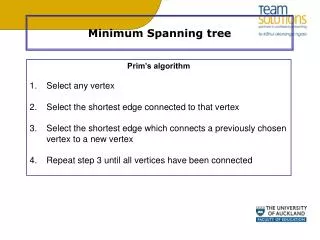
Minimum Spanning Tree Prim’s AlgorithmKruskal’s Algorithm
The Scenario • Construct a telephone network… • We’ve got to connect many cities together • Each city must be connected • We want to minimize the total cable used
The Scenario • Construct a telephone network… • We’ve got to connect many cities together • Each city must be connected • We want to minimize the total cable used
Minimum Spanning Tree • Required: Connect all nodes at minimum cost.
Minimum Spanning Tree • Required: Connect all nodes at minimum cost. 1 3 2
Minimum Spanning Tree • Required: Connect all nodes at minimum cost. • Cost is sum of edge weights 1 1 3 3 2 2
Minimum Spanning Tree • Required: Connect all nodes at minimum cost. • Cost is sum of edge weights 1 1 3 3 2 2 S.T. = 3 S.T. = 5 S.T. = 4
Minimum Spanning Tree • Required: Connect all nodes at minimum cost. • Cost is sum of edge weights 1 1 1 3 3 3 2 2 2 M.S.T. = 3 S.T. = 5 S.T. = 4
Minimum Spanning Tree • Required: Connect all nodes at minimum cost. • Cost is sum of edge weights • Can start at any node