Download
1 / 20
210 likes | 335 Vues
Chapter 18: Spending, Output, and Fiscal Policy. Identify the key assumptions of the basic Keynesian model and explain how this affects firms' production decisions

E N D
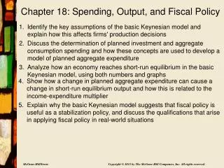
Chapter 18: Spending, Output, and Fiscal Policy Identify the key assumptions of the basic Keynesian model and explain how this affects firms' production decisions Discuss the determination of planned investment and aggregate consumption spending and how these concepts are used to develop a model of planned aggregate expenditure Analyze how an economy reaches short-run equilibrium in the basic Keynesian model, using both numbers and graphs Show how a change in planned aggregate expenditure can cause a change in short-run equilibrium output and how this is related to the income-expenditure multiplier 5.Explain why the basic Keynesian model suggests that fiscal policy is useful as a stabilization policy, and discuss the qualifications that arise in applying fiscal policy in real-world situations
Keynesian Model John Maynard Keynes (1883 – 1946) • After World War I, Keynes recognized that the terms of the peace would lead to another war • Building block for current theories of short-run economic fluctuations and stabilization policies • In the short run, firms meet demand at preset prices • Firms typically set a price and meet the demand at that price in the short run • Menu costs are the costs of changing prices • Firms change prices when the marginal benefits exceed the marginal costs
Planned Aggregate Expenditure PAE = C + IP + G + NX • Planned aggregate expenditure (PAE) is total planned spending on final goods and services • Four components of planned aggregate expenditure • Consumption (C) by households • Investment (I) is planned spending by domestic firms on new capital goods • Government purchases (G) are made by federal, state, and local governments • Net exports (NX) equals exports minus imports
Consumption Function • The consumption function is an equation relating planned consumption to its determinants, notably disposable income (Y – T) C = C + (mpc) (Y – T), where C is autonomous consumption spendingmpc is the change in consumption for a given change in disposable income 0 < mpc < 1 • Autonomous consumption is spending not related to the level of disposable income • A change in C shifts the consumption function
Consumption Function C = C + (mpc) (Y – T) • The wealth effect is the tendency of changes in asset prices to affect household's wealth and thus their consumption spending • This effect is included in C • Autonomous consumption also captures the effects of interest rates on consumption • Higher rates increase the cost of using credit to purchase consumer durables and other items
More on the Consumption Function C = C + (mpc) (Y – T) • Marginal propensity to consume (mpc) is the increase in consumption spending when disposable income increases by $1 • mpc is between 0 and 1 for the economy • If households receive an extra $1 in income, they spend part (mpc) and save part • (Y – T) is disposable income • Output plus government transfers minus taxes • Main determinant of consumption spending
Planned Aggregate Expenditure (PAE) • Two dynamic patterns in the economy • Declines in production lead to reduced spending • Reductions in spending lead to declines in production and income • Consumption is the largest component of PAE • Consumption depends on output, Y • PAE depends on Y • Planned aggregate expenditure has two parts • Autonomous expenditure, the part of spending that is independent of output • Induced expenditure, the part of spending that depends on output (Y)
Short-Run Equilibrium • Short-run equilibrium is the level of output at which planned spending is equal to output • No change in output as long as prices are constant • Our equilibrium condition can be written Y = PAE
Output Greater than Equilibrium Suppose output reaches 5,000 Planned spending is less than total output Unplanned inventory increases Businesses slow down production Output goes down Y = PAE PAE = 960 + 0.8Y PAE 960 45o 4,800 5,000 Output (Y)
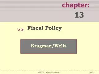
Output Less than Equilibrium Suppose output is only 4,500 Planned spending is more than total output Unplanned inventory decreases Businesses speed up production Output goes up Y = PAE PAE = 960 + 0.8Y PAE 960 4,700 4,800 Output (Y)
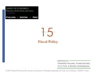
Lower Equilibrium Y = PAE PAE = 960 + 0.8Y PAE = 950 + 0.8Y E Planned aggregate expenditure (PAE) F 960 950 Recessionary gap 45o 4,800 4,750 Y* Output Y
New Equilibrium – • Autonomous consumption, C, decreases by 10 • Causes a downward shift in the planned aggregate expenditure curve • The economy eventually adjusts to a new lower level of equilibrium spending and output, $4,750 • Suppose that the original equilibrium level, $4,800, represented potential output, Y* • A recessionary gap develops • Size of the recessionary gap is 4,800 – 4,750 = $50 • Entire decrease is in consumption spending • Same process applies to a decrease in IP, G, or NX
What Caused U.S. Recession 2007 - 2009 • Housing price bubble burst summer 2006 • House prices increased an average 7% per year from 2001 - 2006 • Last period of high increase was 1976 – 1979 • 4.9% per year increase on average • Using the rule of 72, house prices would double in 10 years as compared to 15-19 years • Housing prices declined 6% 2006 – 2007 and 19% 2007 – 2009 • Financial market crisis
What Caused the U.S. Recession 2007 - 2009 • Decline in spending by businesses and households • Difficult to borrow • Uncertainty about the state of the economy • Decline in planned aggregate expenditure • Downward shift of the PAE line • Recessionary gap
Income-Expenditure Multiplier • The income – expenditure multiplier shows the effect of a one-unit increase in autonomous expenditure on short-run equilibrium output • Previous example • Initial planned expenditure = 960 + 0.8 Y • New planned expenditure = 950 + 0.8 Y • Equilibrium changed from $4,800 to $4,750 • A $10 change in autonomous expenditures caused a $50 change in output • Multiplier = 5 • The larger the mpc, the greater the multiplier
Stabilization Policy • Stabilization policies are government policies that are used to affect planned aggregate expenditure, with the objective of eliminating output gaps • Expansionary policies increase planned expenditure • Contractionary policies decrease planned expenditure • Fiscal policy uses changes in government spending, transfers, or taxes • Monetary policy uses changes in the money supply
Government Spending • Government spending is part of planned spending • Changes in government spending will directly affect planned aggregate expenditures • Suppose planned spending decreases $10 from Y = 960 + 0.8 Y to Y = 950 + 0.8 Y • Equilibrium Y decreases from $4,800 to $4,750 • Recessionary gap is $50 • Stabilization policy indicates a $10 increase in government spending will restore the economy to Y* at $4,800
Taxes and Transfers • Net tax ( T) = total taxes – transfer payments – government interest payments • Planned aggregate expenditures are influenced by changing total taxes and/or transfer payments • The effect is indirect, channeled through the effects on disposable income • Lower taxes or higher transfers increase disposable income • Increases in disposable income lead to higher C
Supply-Side Effects of Fiscal Policy • Fiscal policy may affect potential output as well as potential spending • Investment in infrastructure increases Y* • Taxes and transfers affect incentives and can change potential output, Y* • Supply-side economists emphasize the supply-side effects of fiscal policy • Current thinking is more moderate • Demand-side effects of spending matter • Supply-side effects also matter
Fiscal Policy and Deficit Spending • Government deficit is the difference between government spending and net taxes, (G – T) • Large and persistent budget deficits reduce national saving • Less saving means less investment which means less growth • Managing the impact of the deficit limits the government's ability to use fiscal policy as a stimulus • Political considerations make it difficult to use contractionary fiscal policy • Automaticstabilizers increase government spending or decrease taxes when real output declines • Fiscal policy may be useful to address prolonged periods of recession