Multimedia Data Introduction to Lossless Data Compression

1. Multimedia DataIntroduction to Lossless Data Compression Dr Mike Spann http://www.eee.bham.ac.uk/spannm M.Spann@bham.ac.uk Electronic, Electrical and Computer Engineering

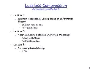
2. Lossless Compression An introduction to lossless compression methods including:- • Run-length coding • Huffman coding • Lempel-Ziv

3. Run-Length Coding (Reminder) Run-length coding is a very simple example of lossless data compression. Consider the repeated pixels values in an image … 000000000000555500000000 compresses to (12,0)(4,5)(8,0) 24 bytes reduced to 6 gives a compression ratio of 24/6 = 4:1 • There must be an agreement between sending compressor and receiving decompressor on the format of the compressed stream which could be (count, value) or (value, count). • We also noted that a source without runs of repeated symbols would expand using this method.

4. Patent Issues There is a long history of patent issues in the field of data compression. Even run length coding is patented. From the comp.compression faq : Tsukiyama has two patents on run length encoding: 4,586,027 and 4,872,009 granted in 1986 and 1989 respectively. The first one covers run length encoding in its most primitive form: a length byte followed by the repeated byte. The second patent covers the 'invention' of limiting the run length to 16 bytes and thus the encoding of the length on 4 bits. Here is the start of claim 1 of patent 4,872,009, just for interest: “A method of transforming an input data string comprising a plurality of data bytes, said plurality including portions of a plurality of consecutive data bytes identical to one another, wherein said data bytes may be of a plurality of types, each type representing different information, said method comprising the steps of: [...]”

5. Huffman Compression • Source character frequency statistics are used to allocate codewords for output. • Compression can be achieved by allocating shorter codewords to the more frequently occurring characters. For example, in Morse code E= • Y= - • - -).

6. Huffman Compression • By arranging the source alphabet in descending order of probability, then repeatedly adding the two lowest probabilities and repeating, a Huffman tree can be generated. • The resultant codewords are formed by tracing the tree path from the root node to the codeword leaf. • Rewriting the table as a tree, 0s and 1s are assigned to the branches. The codewords for each symbols are simply constructed by following the path to their nodes.

7. Huffman Compression

8. Is That All There is to it? • David Huffman invented this method in 1951 while a graduate student of Robert Fano. He did not invent the idea of a coding tree. His insight was that by assigning the probabilities of the longest codes first and then proceeding along the branches of the tree toward the root, he could arrive at an optimal solution every time. • Fano and Shannon had tried to work the problem in the opposite direction, from the root to the leaves, a less efficient solution. • When presented with his student's discovery, Huffman recalls, Fano is said to have exclaimed: "Is that all there is to it!" From the September 1991 issue of Scientific American, pp. 54, 58. Top right – Original figures from IRE Proc. Sept 1952

9. Huffman Compression Questions: • What is meant by the ‘prefix property’ of Huffman? • What types of sources would Huffman compress well and what types would it compress inefficiently? • How would it perform on images or graphics?

10. Static and Adaptive Compression • Compression algorithms remove/exploit source redundancy by using some definition (model) of the source characteristics. • Compression algorithms which use a pre-defined source model are static. • Algorithms which use the data itself to fully or partially define this model are referred to as adaptive. • Static implementations can achieve very good compression ratios for well defined sources. • Adaptive algorithms are more versatile, and update their source models according to current characteristics. However, they have lower compression performance, at least until a suitable model is properly generated.

11. Lempel-Ziv Compression • Lempel-Ziv published mathematical journal papers in 1977 and 1978 on two compression algorithms (these are often abbreviated as LZ’77 and LZ’78) • Welch popularised them in1984 • LZW was implemented in many popular compression methods including .GIF image compression. • It is lossless and universal (adaptive) • It exploits string-based redundancy • It is not good for image compression (why?)

12. Lempel-Ziv Dictionaries How they work :- • Parse data character by character generating a dictionary of previously seen strings • LZ’77 uses a sliding window dictionary • LZ’78 uses a full dictionary history • Refinements added to the LZ’78 algorithm by Terry Welch in 1984 • Known as the LZW algorithm LZ’78 Description • With a source of 8-bits/character (i.e., source values of 0-255.) Extra characters will be needed to describe strings in our dictionary. So we will need more than 8 bits. • Start with output using 9-bits. So now we can use values from 0-511. • We will need to reserve some characters for ‘special codewords’ say, 256-262, so dictionary entries would begin at 263. • We can refer to dictionary entries as D1, D2, D3 etc. (equivalent to 263, 264, 265 etc.) • Dictionaries typically grow to 12- and 15-bit lengths.

13. Lempel-Ziv Compression • LZ’78 Description (cont) • Simple idea of assigning codewords to individual characters and sub-strings which are contained in a dictionary • Pseudocode is relatively simple • BUT careful implementation required to efficiently represent the dictionary • Example - encoding the string ‘THETHREETREES’ STRING = get input character WHILE there are still input characters DO CHARACTER = get input character     IF STRING+CHARACTER is in the string table then         STRING = STRING+character     ELSE         output the code for STRING         add STRING+CHARACTER to the string table         STRING = CHARACTER     END of IF END of WHILE output the code for STRING

14. Lempel-Ziv Compression (Example)

15. Lempel-Ziv Compression • So the compressed output is “THE<D1>RE<D3><D5>ES”. • Each of these 10 output codewords is represented using 9 bits. • So the compressed output uses 90 bits • The original source contains 13x8-bit characters (=104 bits) and the compressed output contains 10x9-bit codewords (=90 bits) • So the compression ratio = (old size/new size):1 = 1.156:1 • So some compression was achieved. Despite the fact that this simple implementation of Lempel-Ziv would normally start by expanding the data, this example has achieved compression. This was because the compressed string was particularly high in repeating strings, which is exactly the type of redundancy the method exploits • For real world data with not so much redundancy, compression doesn't begin until a sizable table has been built, usually after at least one hundred or so characters have been read in

16. Lempel-Ziv Decompression • You might think that in order to decompress a code stream, the dictionary would need to be transmitted first • This is not the case! • A really neat feature of Lempel-Ziv is that the dictionary can be built as the code stream is being decompressed • The reason is that a code for a dictionary entry is generated by the compression algorithm BEFORE it is output into the code stream • The decompression algorithm can mirror this process to reconstruct the dictionary

17. Lempel-Ziv Decompression • Again the pseudo code is quite simple • We can apply this algorithm to the code stream from the compression example to see how it works Read OLD_CODE output OLD_CODE WHILE there are still input characters DO     Read NEW_CODE     STRING = get translation of NEW_CODE     output STRING     CHARACTER = first character in STRING     add OLD_CODE + CHARACTER to the translation table     OLD_CODE = NEW_CODE END of WHILE

18. Lempel-Ziv Decompression (Example)

19. Lempel-Ziv Exercises • Compress the strings “rintintin” and “banananana” • Decompress the string “WHERET<D2>Y<D2><D4><D6><D2>N” (“” represents the space character) • Only for the very keen …. What is the “LZ exception”? • (an example can be found at http://www.dogma.net/markn/articles/lzw/lzw.htm ) • Try decoding the code for banananana

20. This concludes our introduction to selected lossless compression. • You can find course information, including slides and supporting resources, on-line on the course web page at Thank You http://www.eee.bham.ac.uk/spannm/Courses/ee1f2.html

21. rintintin

22. banananana

23. WHERET<D2>Y<D2><D4><D6><D2>N

24. ban<D2><D4><D3>