Comprehensive Overview of Speech & Natural Language Processing
320 likes | 354 Vues
Explore the fundamental concepts and methodologies in Speech and Natural Language Processing, covering areas such as Speech Recognition, Signal Processing, Phonetics, Neural Networks, and Pattern Classification.

Comprehensive Overview of Speech & Natural Language Processing
E N D
Presentation Transcript
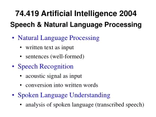
74.419 Artificial Intelligence 2004 Speech &Natural Language Processing • Natural Language Processing • written text as input • sentences (well-formed) • Speech Recognition • acoustic signal as input • conversion into written words • Spoken Language Understanding • analysis of spoken language (transcribed speech)
Speech & Natural Language Processing • Areas in Natural Language Processing • Morphology • Grammar & Parsing (syntactic analysis) • Semantics • Pragamatics • Discourse / Dialogue • Spoken Language Understanding • Areas in Speech Recognition • Signal Processing • Phonetics • Word Recognition
Speech Production & Reception • Sound and Hearing • change in air pressure sound wave • reception through inner ear membrane / microphone • break-up into frequency components: receptors in cochlea / mathematical frequency analysis (e.g. Fast-Fourier Transform FFT) Frequency Spectrum • perception/recognition of phonemes and subsequently words (e.g. Neural Networks, Hidden-Markov Models)
Speech Recognition Phases • Speech Recognition • acoustic signal as input • signal analysis - spectrogram • feature extraction • phoneme recognition • word recognition • conversion into written words
Speech Signal • Speech Signal • composed of different (sinus) waves with different frequencies and amplitudes • Frequency- waves/second like pitch • Amplitude - height of wave like loudness • + noise (not sinus wave) • Speech Signal • composite signal comprising different frequency components
Waveform (fig. 7.20) Amplitude/ Pressure Time "She just had a baby."
Waveform for Vowel ae(fig. 7.21) Amplitude/ Pressure Time Time
Speech Signal Analysis • Analog-Digital Conversion of Acoustic Signal • Sampling in Time Frames (“windows”) • frequency = 0-crossings per time frame • e.g. 2 crossings/second is 1 Hz (1 wave) • e.g. 10kHz needs sampling rate 20kHz • measure amplitudes of signal in time frame • digitized wave form • separate different frequency components • FFT (Fast Fourier Transform) • spectrogram • other frequency based representations • LPC (linear predictive coding), • Cepstrum
Waveform and LPC Spectrum for Vowel ae(figs. 7.21, 7.22) Amplitude/ Pressure Time Energy Formants Frequency
Speech Signal Characteristics From Signal Representation derive, e.g. • formants - dark stripes in spectrum strong frequency components; characterize particular vowels; gender of speaker • pitch– fundamental frequency baseline for higher frequency harmonics like formants; gender characteristic • change in frequency distribution characteristic for e.g. plosives (form of articulation)
Video of glottis and speech signal in lingWAVES (from http://www.lingcom.de)
Phoneme Recognition Recognition Process based on • features extracted from spectral analysis • phonological rules • statistical properties of language/ pronunciation Recognition Methods • Hidden Markov Models • Neural Networks • Pattern Classification in general
Pronunciation Networks / Word Models as Probabilistic FAs (fig 5.12)
Word Recognition with Probabilistic FA / Markov Chain (fig 5.14)
Viterbi-Algorithm - Overview (cf. Jurafsky Ch.5) The Viterbi Algorithm finds an optimal sequence of states in continuous Speech Recognition, given an observation sequence of phones and a probabilistic (weighted) FA (state graph). The algorithm returns the path through the automaton which has maximum probability and accepts the observation sequence. a[s,s'] is the transition probability (in the phonetic word model) from current state s to next state s', and b[s',ot] is the observation likelihood of s' given ot. b[s',ot] is 1 if the observation symbol matches the state, and 0 otherwise.
Viterbi-Algorithm (fig 5.19) function VITERBI(observations of len T, state-graph) returns best-path num-statesNUM-OF-STATES(state-graph) Create a path probability matrix viterbi[num-states+2,T+2] viterbi[0,0]1.0 for each time step tfrom 0to Tdo for each state sfrom 0 to num-statesdo for each transition s'from s in state-graph new-score viterbi[s,t] * a[s,s'] * b[s',(ot)] if ((viterbi[s',t+1] = 0) || (new-score > viterbi[s',t+1])) then viterbi[s',t+1]new-score back-pointer[s',t+1]s Backtrace from highest probability state in the final column of viterbi[]and return path word model observation (speech recognizer)
Viterbi-Algorithm Explanation (cf. Jurafsky Ch.5) • The Viterbi Algorithm sets up a probability matrix, with one column for each time index t and one row for each state in the state graph.Each column has a cell for each state qi in the single combined automaton for the competing words (in the recognition process). • The algorithm first creates N+2 state columns. The first column is an initial pseudo-observation, the second corresponds to the first observation-phone, the third to the second observation and so on. The final column represents again a pseudo-observation. In the first column, the probability of the Start-state is initially set to 1.0; the other probabilities are 0. Then we move to the next state. For every state in column 0, we compute the probability of moving into each state in column 1. The value viterbi[t, j] is computed by taking the maximum over the extensions of all the paths that lead to the current cell. An extension of a path at state i at time t-1 is computed by multiplying the three factors: • the previous path probability from the previous cell forward[t-1,i] • the transition probabilityai,j from previous state i to current state j • the observation likelihood bjt that current state j matches observation symbol t. bjtis 1 if the observation symbol matches the state; 0 otherwise.
Speech Recognition Acoustic / sound wave Filtering, Sampling Spectral Analysis; FFT Frequency Spectrum Features (Phonemes; Context) Signal Processing / Analysis Phoneme Recognition: HMM, Neural Networks Phonemes Grammar or Statistics Phoneme Sequences / Words Grammar or Statistics for likely word sequences Word Sequence / Sentence
Speech Processing - Important Types and Characteristics single word vs. continuous speech unlimited vs. large vs. small vocabulary speaker-dependent vs. speaker-independent training Speech Recognition vs. Speaker Identification
Additional References Hong, X. & A. Acero & H. Hon: Spoken Language Processing. A Guide to Theory, Algorithms, and System Development. Prentice-Hall, NJ, 2001 Figures taken from: Jurafsky, D. & J. H. Martin, Speech and Language Processing, Prentice-Hall, 2000, Chapters 5 and 7. lingWAVES (from http://www.lingcom.de