Clustering and Network
1. Clustering and Network. Park, Jong Hwa MRC-DUNN Hills Road Cambridge CB2 2XY England. Bioinformatics in Biosophy. Next :. 02/06/2001. Clustering of data is a method by which large sets of data is grouped into clusters of smaller sets of similar data. What is clustering?.

Clustering and Network
E N D
Presentation Transcript
1 Clustering and Network Park, Jong Hwa MRC-DUNN Hills Road Cambridge CB2 2XY England Bioinformatics in Biosophy Next: 02/06/2001
Clustering of data is a method by which large sets of data is grouped into clusters of smaller sets of similar data. What is clustering? we see clustering means grouping of data or dividing a large data set into smaller data sets of some similarity. http://cne.gmu.edu/modules/dau/stat/clustgalgs/clust1_frm.html http://www-cse.ucsd.edu/~rik/foa/l2h/foa-5-4-2.html
What is a clustering algorithm ? A clustering algorithm attempts to find natural groups of components (or data) based on some similarity. The clustering algorithm also finds the centroid of a group of data sets. To determine cluster membership, most algorithms evaluate the distance between a point and the cluster centroids. The output from a clustering algorithm is basically a statistical description of the cluster centroids with the number of components in each cluster.
Error function is a function that indicates quality of clustering Definition: The centroid of a cluster is a point whose parameter values are the mean of the parameter values of all the points in the clusters.
What is the common metric for clustering techniques ? Generally, the distance between two points is taken as a common metric to assess the similarity among the components of a population. The most commonly used distance measure is the Euclidean metric which defines the distance between two points p= ( p1, p2, ....) and q = ( q1, q2, ....) as :
For sequence comparison, the distances can be genetic distance (such as PAM) For clustering Expression profiles, euclidean distance can be used. Distances are defined according to problems.
Kinds of Clustering algorithms Non-hierarchical clustering methods Single-pass methods Reallocation methods K-means clustering Hierarchical clustering methods Group average link method (UPGMA) Single link method MST Algorithms complete link method Voorhees AlgorithmWard's method (minimum variance method) Centroid and median methods General algorithm for HACM
Hierarchical Clustering Dendrograms used for representation. • General Strategy is to represent similarity matrix as a graph, form a separate cluster around each node, and traverse the edges in decreasing order of similarity, merging two clusters according to some criterion. • Merging criteria: • Single-link : Merge maximally connected components. • Minimum Spanning Tree based approach: merge clusters connected by MST edge with smallest weight. • Complete-link : Merge to get a maximally complete component.
Partitional: Single partition is found. Hierarchical: Sequence of nested partitions is found, by merging two partitions at every step. • Agglomerative: glue together smaller clusters • Divisive: fragment a larger cluster into smaller ones.
Partitional Clustering Find a single partition of k clusters based on some clustering criteria. • Clustering criteria: • local : forms clusters by utilizing local structure in the data. (e.g. Nearest neighbor clustering) • global: represents each cluster by a prototype and assigns a pattern to a cluster with most similar prototype. (e.g. K-means, Self Organizing Maps) • Many other techniques in literature such as density estimation and mixture decomposition. • From [Jain & Dubes] Algorithms for Clustering Data, 1988
Nearest Neighbor Clustering • Input: • A threshold, t, on the nearest-neighbor distance. • Set of data points {x1, x2, ? xn}. • Algorithm: • [Initialize: assign x1 to cluster C1. Set i = 1, k = 1. • Set i = i+1. Find nearest neighbor of xi among the patterns already assigned to clusters. • Let the nearest neighbor be in cluster m. If its distance > t, then increment k and assign xi to a new cluster Ck; else assign xi to Cm. • If every data point is assigned to a cluster, then stop; else go to first step above. • From [Jain & Dubes] Algorithms for Clustering Data, 1988
Iterative Partitional Clustering Input: • K, number of clusters; Set of data points {x1, x2, ,, xn}; • a measure of distance between them (e.g. Euclidean, Mahalanobis); and clustering criterion (e.g. minimize squared error) Algorithm: • [Initialize: A random partition with K cluster-centers.] • Generate a new partition by assigning each data point to its closest cluster center. • Compute new cluster centers as centroids of the clusters. • Repeat above two steps until optimum value of criterion found. • Finally, adjust the number of clusters by merging/splitting existing clusters, or by removing small (outlier) clusters. • From [Jain & Dubes] Algorithms for Clustering Data, 1988
AVERAGE LINKAGE CLUSTERING: The dissimilarity between clusters is calculated using average values. Unfortunately, there are many ways of calculating an average! The most common (and recommended if there is no reason for using other methods) is UPGMA - Unweighted Pair-Groups Method Average. The average distance is calculated from the distance between each point in a cluster and all other points in another cluster. The two clusters with the lowest average distance are joined together to form the new cluster. (Sneath, P.H.A. and Sokal, R.R. (1973) in Numerical Taxonomy (pp; 230-234), W.H. Freeman and Company, San Francisco, California, USA)
The GCG program PILEUP uses UPGMA to create its dendrogram of DNA sequences, and then uses this dendrogram to guide its multiple alignment algorithm. The GCG program DISTANCES calculates pairwise distances between a group of sequences.
COMPLETE LINKAGE CLUSTERING (Maximum or Furthest-Neighbour Method): The dissimilarity between 2 groups is equal to the greatest dissimilarity between a member of cluster i and a member of cluster j.
Furthest Neighbour This method tends to produce very tight clusters of similar cases.
SINGLE LINKAGE CLUSTERING (Minimum or Nearest-Neighbour Method): The dissimilarity between 2 clusters is the minimum dissimilarity between members of the two clusters. This methods produces long chains which form loose, straggly clusters. This method has been widely used in numerical taxonomy.
WITHIN GROUPS CLUSTERING This is similar to UPGMA except clusters are fused so that within cluster variance is minimised. This tends to produce tighter clusters than the UPGMA method. UPGMA: Unweighted Pair-Groups Method Average
Ward’smethod Cluster membership is assessed by calculating the total sum of squared deviations from the mean of a cluster. The criterion for fusion is that it should produce the smallest possible increase in the error sum of squares. Lance, G. N. and Williams, W. T. 1967. A general theory of classificatory sorting strategies. Computer Journal, 9: 373-380.
K-Means Clustering Algorithm This nonheirarchial method initially takes the number of components of the population equal to the final required number of clusters. In this step itself the final required number of clusters is chosen such that the points are mutually farthest apart. Next, it examines each component in the population and assigns it to one of the clusters depending on the minimum distance. The centroid's position is recalculated everytime a component is added to the cluster and this continues until all the components are grouped into the final required number of clusters.
Complexity of K-means Algorithm • Time Complexity = O(RKN) • Space Complexity = O(N) where R is the number of iterations
K-Medians AlgorithmK-medians algorithm is similar to K-means algorithm except it uses a median instead of a mean Time Complexity = O(RN2) where R is the number of iterations Space Complexity = O(N)
K-Means VS. K-Medians (1) • K-means algorithm requires a continuous space, so that a mean is a potential element of space • K-medians algorithm also works in discrete spaces where a mean has no meaning • K-means requires less computational time because it is easier to compute a mean than to compute a median
Problems with K-means Clustering • To achieve a globally minimum error is NP-Complete • Very sensitive to initial points • When used with large databases, time complexity can easily become intractable • Existing algorithms are not generic enough to detect various shapes of clusters (spherical, non-spherical, etc.)
Genetic Clustering Algorithm • Genetic Clustering Algorithms * achieve a “better” clustering result than K-Means • Refining the initial points * achieve a “better” local minimum and reduce convergent time
A Genetic Clustering Algorithm • "Clustering using a coarse-grained parallel Genetic Algorithm: A Preliminary Study", N. K. Ratha, A. K. Jain, and M. J. Chung, IEEE, 1995 • Use a genetic algorithm to solve a K-means clustering problem formulated as an optimization problem • We can also look at it as a label assignment problem such that the assignment of {1,2,…,K} to each pattern minimizes the similarity function.
Definition of Genetic Algorithm • Search based on the “survival of the fittest” principle [R.Bianchini and et al.,1993] • The “fittest candidate” is the solution at any given time. • Run the evolution process for a sufficiently large number of generations
Simple Genetic Algorithm Function GENETIC-ALGO(population, FITNESS-FN) returns an individual inputs: population, a set of individuals (fixed number) FITNESS-FN, a function that measures the fitness of an individual repeat parents = SELECTION(population, FITNESS-FN) population = REPRODUCTION(parents) until some individual is fit enough return the best individual in population, according to FINESS-FN
Pros and Cons Pros • Clustering results are better as compared to K-means algorithm. Cons • Search space grows exponentially as a function of the problem size. • Parallel computing helps but not much
Need for better clustering algorithms. Enormity of data • hierarchical clusterings soon become impractical High Dimensionality • Distance based algorithms become ill-defined because of the curse of dimensionality. • Collapse of notion neighborhood --> physical proximity. • All the data is far from the mean! Handling Noise • Similarity measure becomes noisy as the hierarchical algorithm groups more and more points, hence clusters that should not have been merged may get merged!
Handling High Dimensionality • Reduce the Dimensionality and apply traditional techniques. • Dimensionality Reduction: • Principal Component Analysis (PCA), Latent Semantic Indexing (LSI): • Use Singular Value Decomposition (SVD) to determine the most influential features (maximum eigenvalues) • Given data in a n x m matrix format (n data points, m attributes), PCA computes SVD of a covariance matrix of attributes, whereas LSI computes SVD of original data matrix. LSI is faster and memory efficient, and has been successful in information retrieval domain (clustering documents). • Multidimensional Scaling (MDS): • Preserves original rank ordering of the distances among data points.
Clustering in High Dimensional Data Sets DNA /Protein/ Interaction data are high-dimentional. • Traditional distance-based approach • Hypergraph-based approach
Hypergraph-Based Clustering • Construct a hypergraph in which related data are connected via hyperedges. • How do we find related sets of data items? Use Association Rules! • Partition this hypergraph in a way such that each partition contains highly connected data.
graph • Definition: A set of items connected by edges. Each item is called a vertex or node. Formally, a graph is a set of vertices and a relation between vertices, adjacency. • See alsodirected graph, undirected graph, acyclic graph, biconnected graph, connected graph, complete graph, sparse graph, dense graph, hypergraph, multigraph, labeled graph, weighted graph, self-loop, isomorphic, homomorphic, graph drawing, diameter, degree, dual, adjacency-list representation, adjacency-matrix representation. • Note: Graphs are so general that many other data structures, such as trees, are just special kinds of graphs. Graphs are usually represented G = (V,E), where V is the set of vertices, and E is the set of edges. If the graph is undirected, the adjacency relation is symmetric. If the graph does not allow self-loops, adjacency is irreflexive. • A graph is like a road map. Cities are vertices. Roads from city to city are edges. (How about junctions or branches in a road? You could consider junctions to be vertices, too. If you don't want to count them as vertices, a road may connect more than two cities. So strictly speaking you have hyperedges in a hypergraph. It all depends on how you want to define it.) • Another way to think of a graph is as a bunch of dots connected by lines. Because mathematicians stopped talking to regular people long ago, the dots in a graph are called vertices, and the lines that connect the dots are called edges. The important things are edges and the vertices: the dots and the connections between them. The actual position of a given dot or the length or straightness of a given line isn't at issue. Thus the dots can be anywhere, and the lines that join them are infinitely stretchy. Moreover, a mathematical graph is not a comparison chart, nor a diagram with an x- and y-axis, nor a squiggly line on a stock report. A graph is simply dots and lines between them---pardon me, vertices and edges. Michael Bolton <mb@michaelbolton.net> 22 February 2000
Graph • Formally a graph is a pair (V,E) where V is any set, called the vertex set, and the edge setE is any subset of the set of all 2-element subsets of V. Usually the elements of V, the vertices, are illustrated by bold points or small circles, and the edges by lines between them.
hypergraph • Definition: A graph whose hyperedges connect two or more vertices. • See alsomultigraph, undirected graph. • Note: Consider ``family,'' a relation connecting two or more people. If each person is a vertex, a family edge connects the father, mother, and all of their children. So G = (people, family) is a hypergraph. Contrast this with the binary relations ``married to,'' which connects a man and a woman, or ``child of,'' which is directed from a child to his or her father or mother.
General Approach for High Dimensional Data Sets • Data • Graph • Sparse Hypergraph • Sparse Graph • Association Rules • Similarity • measure • Partitioning based • Clustering • Agglomerative • Clustering
references • [1] Usama Fayyad, Gregory Piatetsky-Shapiro, Padhraic Smyth, and Ramasamy Uthurasamy (eds.), Advances in Knowledge Discovery and Data Mining, AAAI Press/ The MIT Press, 1996. • [2] Michael Berry and Gordon Linoff, Data Mining Techniques (For Marketing, Sales, and Customer Support), John Wiley & Sons, 1997. • [3] Sholom M. Weiss and Nitin Indurkhya, Predictive Data Mining (a practical guide), Morgan Kaufmann Publishers,1998. • [4] Alex Freitas and Simon Lavington, Mining Very Large Databases with Parallel Processing, Kluwer Academic Publishers, 1998. • [5] A. K. Jain and R. C. Dubes, Algorithms for Clustering Data, Prentice Hall, 1988. • [6] V. Cherkassky and F. Mulier, Learning from Data, John Wiley & Sons, 1998. • [7] Vipin Kumar, Ananth Grama, Anshul Gupta, and George Karypis, Introduction to Parallel Computing: Algorithm Design and Analysis, Benjamin Cummings/Addison Wesley, Redwood City, 1994. • Research Paper References: • [1] J. Ross Quinlan, C4.5: Programs for Machine Learning, Morgan Kaufmann, 1993. • [2] M. Mehta, R. Agarwal, and J. Rissanen, SLIQ: A Fast Scalable Classifier for Data Mining, Proc. Of the fifth Int. Conf. On Extending Database Technology (EDBT), Avignon, France, 1996. • [3] J. Shafer, R. Agrawal, and M. Mehta, SPRINT: A Scalable Parallel Classifier for Data Mining, Proc. 22nd Int. Conf. On Very Large Databases, Mumbai, India, 1996.
Gene expression and genetic network analysis A gene’s expression level is the number of copies of that gene’s RNA produced in a cell, and correlates with the amount of the corresponding protein produced DNA microarrays greatly improve the scalability and accuracy of gene expression level monitoring – can simultaneously monitor 1000’s of gene expression levels http://www.ib3.gmu.edu/gref/S01/csi739/overview.pdf
Goals of Gene Expression Analysis What genes are or are not expressed? Correlate expression with other parameters • – developmental state • – cell types • – external conditions • – disease states Outcome of analysis • – Functions of unknown genes • – Identify co-regulated groups • – Identify gene regulators and inhibitors • – Environmental impact on gene expression • – Diagnostic gene expression patterns
Methods for Gene Expression Analysis Early processing: • – image analysis • – statistical analysis of redundant array elements • – output raw or normalized expression levels • – store results in database Clustering • – visualization • – unsupervised methods • – supervised methods Modeling • – reverse engineering • – Genetic network inference
Unsupervised Clustering Methods Direct visual inspection • – Carr et al (1997) Stat Comp Graph News 8(1) • – Michaels et al (1998) PSB 3:42-53 Hierarchical clustering • – DeRisi et al (1996) Nature Genetics 14: 457-460 Average linkage • – Eisen et al (1998) PNAS 95:14863-14868 • – Alizadeh (2000) Nature 403: 503-511 k-means • – Tavazoie et al (1999) Nature Genetics 22:281-285
Unsupervised Clustering Methods SOMs • – Toronen et al (1999) FEBS Letters 451:142-146 • – Tamayo et al (1999) PNAS 96:2907-2912 Relevance networks • – Butte et al (2000), PSB 5: 415-426 SVD/PCA • – Alter et al (2000) PNAS 97(18):10101-10106 Two-way clustering • – Getz et al (2000) PNAS 97(22):12079-12084 • – Alon et al (1999) PNAS 96:6745-6750
Supervised Learning Goal: classification • – genes • – disease state • – developmental state • – effects of environmental signals Linear discriminant Decision trees Support vector machines • – Brown et al (2000) PNAS 97(1) 262-267