Create Effective Charts in Excel: A Comprehensive Guide for Data Visualization
This lesson covers the essentials of creating various types of charts in Excel, including pie charts, column charts, line graphs, and scatter plots. You'll learn how to select data, insert charts, and customize their design to effectively visualize your data insights. The tutorial also addresses common issues like data labels and axis labels, providing solutions to enhance your charts. Whether you're illustrating proportions or analyzing trends over time, mastering these charting techniques will elevate your data presentations.

Create Effective Charts in Excel: A Comprehensive Guide for Data Visualization
E N D
Presentation Transcript
Charts and Graphs Topic 7: Visualization Lesson 1 – Creating Charts in Excel
Charts Data is often better explained through visualization as either a graph or a chart. Excel makes creating charts easy: Column Charts Pie Charts Bar Graphs Line Graphs Area Graphs Scatter Plots Charts can be found on the Insert Tab
Sample Data Here’s some sales data that we would like to visualize:
Pie Charts A pie chart is useful when you are trying to show proportions. How much of the sales revenue comes from each client? Who are our largest clients?
Creating a Pie Chart Select the data and the headers Go to Insert tab Within the Charts section, click on Pie Then select a type of pie chart jys
Customizing a Chart Use the Chart Tools Tabs to customize a Chart Design Tab Format Tab
A Customized Version of the Same Pie Chart Use the Design tab to change the look of the Chart or to Add additional chart elements Use the Format tab to rearrange items in the chart
Transparency creates a Minimal Display Choosing a transparent background for a chart is useful for creating a worksheet that minimizes chart details and simply shows a small graphic to support a set of numbers
Other Formatting Options The ‘+’ icon allows you to add a new chart element The paintbrush icon allows you to change the format of the item The funnel icon allows you to limit the data in the chart Format panel allows you to customize any chart element selected
Column Chart Also known as a bar chart, with rectangular bars of lengths usually proportional to the magnitudes or frequencies of what they represent. The bars are vertically oriented in a column chart Useful for showing data changes over a period of time, or illustrating comparisons of groups Categories organized on horizontal axis Values on vertical axis
Column chart Same data, different chart type
Line Graph Often used to plot changes in data over time such as weekly temperature changes or stock market prices If plotting changes over time: Time is plotted along the horizontal or x-axis Data is plotted as individual points along the vertical axis
High, Low, Close Graph Used to illustrate the fluctuation of stock prices or for scientific data The data should be arranged with stock names as row headings, and High, Low and Close entered as column headings In “Stock” Charts in Excel
X/Y Scatter Plot Useful for determining how two variables relate to one another e.g. profits vs. expenditures, height vs. weight, etc. Each data point has more than one attribute Person (height, weight) Quarter (profit, expenditure) Each attribute on a single axis
Assigning a Series to a Secondary Axis A secondary value axis can make it easier to compare data series that have deviating ranges. Example: a series showing number of units sold per year has a range that is much higher than cost per unit per year. The difference in range makes it difficult to see how they relate to each other. Putting one of the series on a secondary axis makes it possible to compare the variables
Assigning a Series to a Secondary Axis The line graph on the left shows two data series with widely differing ranges, so it’s hard to compare them. The graph on the right, plots one series on a secondary axis making it easier to compare and identify the inverse relationship. To move a series to a secondary axis, right-click on the series, click Format Data Series, select Series Options then select Secondary Axis.
Trendlines, Error Bars, etc. Excel also provides statistical analysis tools via the Design tab / Add Chart Element icon (Excel 2013, 2016) or the Layout tab / Analysis section (Excel 2010) . Trendlines show the “best fit” for the data. Error bars show “confidence intervals” around data points.
Sparklines New to Excel 2010, we can also create charts or graphs that live within one cell Their inventor, Edward Tufte, describes them as “intense, simple, word-sized graphics” Meant to be embedded into what they are describing Presents the general shape of variation in some measurement, in a simple and highly condensed way
To Create Sparklines: Select the cell where you want the Sparkline to appear Click the Insert tab andlook for the Sparklines group Choose the data range and the location for the Sparkline.
Merging Cells To make sparklines bigger, you can merge multiple cells into a single cell. In the home tab:
Common Issues: data labels Data labeled “Series1”
Common Issues: data labels Data labeled “Series1” To fix it: Select Data
Common Issues: data labels Data labeled “Series1” To fix it: Select Data Edit Series Name
Common Issues: axis labels Axis labels plotted instead
Common Issues: axis labels Axis labels plotted instead To fix it: Select Data
Common Issues: Axis Labels Axis labels plotted instead To fix it: Select Data Remove axis series Edit Axis Labels