Download

1 / 25
250 likes | 359 Vues
This research by David Lomet and Mark Tuttle presents a simpler approach to efficient redo recovery in databases. The proposed method eliminates the need for managing conflicting orders and irrelevant variables. By utilizing Conflict and Installation State Graphs, the system ensures recoverable states through a Redo Test and Recovery Procedure.

E N D
A Theory of Redo Recovery David Lomet Microsoft Research, Redmond Mark Tuttle HP Research, Cambridge
Big Picture • Much simpler than our VLDB’95 paper • Redo Recovery requires • Good db state • Replay of the right operations • Good state updates: conflict order not required • Write-read conflicts can be ignored • Some db “variables” irrelevant (don’t need to update them) • Synchronize State update & ops replayed • Captured in recovery Invariant • We prove that maintaining invariant recovery • Current recovery methods: maintain invariant • Show how current methods work (e.g. ARIES redo) • Show how “new” methods could work
Conflict State Graph (CSG) • Conflict graph(“Borrowed” from Concurrency Control) • Nodes are log operations; Edges: conflicts (RW, WR, WW) • State graph SG • Add writes(node): {<name, value>…} of vars updated • State for SG: {<x,v>| <x,v> in writes(n) and n is last node in state graph with x in vars(n)} • Final state Sfinalof CSG is desired recovered state • Any prefix of a state graph is a state graph • Prefix: node in prefix predecessor in prefix • State of any prefix of CSG can be recovered by • Replaying operations in suffix in conflict graph order We will relax CSG requirements
x=0,y=0 x=1,y=0 x=1, y=2 Sfinal : x=3, y=2 Conflict State Graph & States O: readset{x} writes{<x,1>} Write-read edge Write-read & write-write & read-write edge P: readset{x} writes{<y,2>} Q: readset{x} writes{<x,3>} Read-write edge
Installation Graph y written by P • Example: Initial stable state: {<x,0><y,0>} • O: x ← x+1 • P: y ← x+1 • After O,P, state is {<x,1>,<y,2>} • Flush y to disk- Stable state is {<x,0><y,2>} • Replay O- generates correct state {<x,1>,<y,2>} • O’s readset x unchanged by P’s installation • Even though Write-Read edge orders P after O • Installation graph: • conflict graph without write-read edges • Installation state graph (ISG): • same writes(n)for node n as conflict state graph • State of any prefix of ISG can be recovered • More prefixes (states) because of fewer edges
Installation State Graph & States x=0,y=0 O: readset{x} writes{<x,1>} Removed write-read edge x=1,y=0 ISG recoverable state Retained write-write & read-write edge P: readset{x} writes{<y,2>} x=0,y=2 x=1, y=2 Q: readset{x} writes{<x,3>} Retained read-write edge x=3, y=2
Exposed Variables • Example • O1: x ← z+1 • O2: x ← 25 • After O2, we don’t care about x value of O1 • Variable x is unexposed after ops I ({O1} here) if • minconflict op in Ops(log) – I writes x • Without reading it • x’s value is a “don’t care” when x is unexposed • This is example of Physical Logging • Prefix of installation graphexplains state S if values of exposed variables in S are the same as values in state of prefix of ISG
Potentially Recoverable State • Potentially recoverable state: state that • by the replay of a subset of operations of the conflict graph, in conflict order, will produce the recovered state Sfinal • Theorem:If S is a state explained by a prefix of the installation graph, then S is potentially recoverable
REDO Test & Recovery Procedure • REDO: tests op’s in conflict order log scan • Yes (true): replay operation • No (false): bypass operation • redo_set = {O|REDO(O..) & O on scanned log} • Recover Procedure: • Set log scan point to “checkpoint” • while not at log end • O ← current log operation • State = ifREDO(O,State,Log,Analysis) • Then O(State) • Else State • Advance log scan point to next operation • End
Recovery • Recoverable system: a system with • a potentially recoverable state Spot • Replay of O’s in redo_set from Spot produces Sfinal • Inv: ops(Log)-redo_setdefines prefix of the installation state graph that explains State • Every system change must be atomic transition maintaining Inv • Corollary:Given a state,log,checkpoint, and an execution ofRecover (identifying redo_set) • If Inv holds • Then System is recoverable Only specific potentially recoverable state is recoverable
Write Graph • Write graph: start from installation state graph • Collapse set of nodes (acyclic) merges nodes • Add new node for next operation • Add edge (collapse cycles) • Remove a write of an unexposed variable • We do not care about values of unexposed variables • Write graph captures entire system state • Prefix that is stable • Suffix in cache • Cache Manager uses write graph • To maintain potentially recoverable state • Usually by collapsing suffix node into stable prefix
Collapsed Node n x=1, y=2 x=1, y=0 Write Graph {via Node Collapse}Fewer States x=0,y=0 O: readset{x} writes{<x,1>} Removed write-read edge Write graph remains acyclic Based on installation graph Ops(n) = {O,P} Writes(n) = {<x,3>} P: readset{x} writes{<y,2>} x=0,y=2 Q: readset{x} writes{<x,3>} Retained read-write edge translates to flush order for cache manager Keep only one version of each variable in cache x=3, y=2
Stable State Write Graph Prefix Usually Single Node O3 O1 O2 Managing Recovery Updating State Log O1 Atomic O2 Collapse to “Install” X O3 Volatile State Suffix of Write Graph In Cache Removing O3 from redo_set
Physiological Recovery Physical and Logical Recovery described in paper • Physiological recovery (e.g. ARIES) • Operation Form:read A, write A • Log Op has LSN • Variable tagged: LSN of last log op writing it • REDO: op’s LSN > variable LSN “Yes” (Replay) • Our explanation • Ops writing variable collapsed to one cache node • Flushing page to stable state (root of write graph) • Collapses cache node into stable state node • Keeps state potentially recoverable • redo test node’s ops removed from redo_set • Maintains invariant Inv • [state change; redo_set change] is atomic
Extended LSN Method • Generalize physiological ops • read/write multiple variables • Our example: ops can read X, write Y (like P) • also read X, write X • LSNs still effective for REDO test • Flush synchronizes change to state and redo_set • Cache management • Now requires flush of one variable before another • Our theory captures this careful write requirement • Consider B-tree split: (Blink-tree) * • Next slide shows “half split” graphically • Must also post index term for new node
O: readset{x} writes{<x,1>} Collapsed Node Ops(n) = {O,P} Writes(n) = {<x,3>} x=1, y=2 x=1, y=0 Q: readset{x} writes{<x,3>} Extended Recovery {Blink-tree Split} Old Node X New Node Y x=0,y=0 Update Node X Move half to node Y Read X, write Y P: readset{x} writes{<y,2>} x=0,y=2 Flush Y before X In SqlServer 6.0 Update node X remove Y records x=3, y=2
Recoverable Systems Summary • Cache management keeps state potentially recoverable • Very generally via write graph • Derived from installation state graph • Maintains invariant INV • so that replayed operations are correct set • By synchronizing changes to redo_set with changes to state
Outline • Foundation • Conflict graph, state graphs, recovered state • Abstract Recovery • Cache Management: maintaining state • Installation order: weaker update order than conflict order • Recovery • Recovery procedure, redo test • Invariant:guarantees correct recovery • Coordinating state before failure with recovery execution after failure • Recoverable Systems • Write graphs for maintaining potentially recoverable state • Maintaining recovery invariant • Explaining current recovery methods
Managing the Cache • Stable state: prefix of write graph • Usually a single node • Means stable state potentially recoverable • Cache: usually contains write graph suffix • Volatile state- which is lost during system crash • Usually collapsing nodes so that one node per “variable” • State update: move a minimum write graph node in cache to stable state atomically • Start with potentially recoverable state • Atomic transition – frequently node collapse • New potentially recoverable state
Maintaining Recovery Invariant • Potentially recoverable state only “half” of job • Ops(log) – Redo_set must explain state • Jobs need to be synchronized to enforce INV • Examples: Stable state is root of write graph • Logical recovery (in paper) • Physical recovery (in paper) • Physiological recovery * • Extended recovery *
Logical Recovery • Logical recovery with arbitrary log ops — System R • Quiesce and write shadow “checkpoint” to disk • By dumping cache contents to disk shadow pages • Disk shadow is installed atomically • Replacing old versions of shadow variables • Our explanation • Shadow coalesced on disk is single write graph node • Encompassing all changes from last checkpoint • Hence is a write graph prefix • Shadow “installed” atomically” via pointer swing • Accomplished by writing new pointer in checkpoint record to log • Log is truncated with the writing checkpoint record • All prior records are added to checkpoint • Which “installs” all earlier operations simultaneously with stable state update, hence maintaining Inv
Physical Recovery • Physical recovery writes entire page • Pages are written back to disk • When prefix of log contains only pages already written back, log is truncated • Via checkpoint record indicating redo pass start • All records scanned during recovery are replayed • REDO(op) always is “yes” • Our explanation • Operations are blind writes of single variable- read set is empty • All variables with operations not in checkpoint are unexposed • These operations are replayed during recovery • They never read • Writing to those variables leaves them unexposed • However, they are now set to be installed • Installation occurs when checkpoint record is written • Operations now not part of redo scan are thus installed
Our Goal • REDO Recovery explanation (Not all of recovery) • Cache management: stage data to stable state • Goal: fewer writes & less constrained order • Some methods require careful write ordering– why? • Recovery: which ops to replay • And how to coordinate state changes with replay changes • Provably ensure “recoverability” • Disclaimers • Abstract story- real recovery needs more • Simpler operation model than past work • Not everything is explained: • All actually used recovery techniques are handled • But not all recovery techniques we know of are “quite” captured
System Model • State: {<name, value>…} • Operation: • readset(O): set of variables read by O • writeset(O): set of variables written by O • Operations are atomic– system must ensure atomicity • Operation Sequence • Sequence of ops O1,O2,…Ok … Ofinal • State Sequence • Sequence of states S1, S2,… Sk … Sfinal generated by op seg from S0 • Ok precedes (leads to) Sk when executed “against” Sk-1 • Recovery goal • From some state and a record of operations (on log) • Reproduce last state in sequence Sfinal