Download
1 / 36
360 likes | 557 Vues
Biostatistics course Part 16 Lineal regression. Dr. Sc. Nicolas Padilla Raygoza Department of Nursing and Obstetrics Division Health Sciences and Engineering Campus Celaya Salvatierra University of Guanajuato. Biosketch. Medical Doctor by University Autonomous of Guadalajara.

E N D
Biostatistics coursePart 16Lineal regression Dr. Sc. Nicolas Padilla Raygoza Department of Nursing and Obstetrics Division Health Sciences and Engineering Campus Celaya Salvatierra University of Guanajuato
Biosketch Medical Doctor by University Autonomous of Guadalajara. Pediatrician by the Mexican Council of Certification on Pediatrics. Postgraduate Diploma on Epidemiology, London School of Hygiene and Tropical Medicine, University of London. Master Sciences with aim in Epidemiology, Atlantic International University. Doctorate Sciences with aim in Epidemiology, Atlantic International University. Associated Professor B, Department of Nursing and Obstetrics, Division of Health Sciences and Engineering, University of Guanajuato, Campus Celaya Salvatierra, Mexico. padillawarm@gmail.com
Competencies • The reader will know how plot a regression line • He (she) will apply a hypothesis test on regression line • He (she) will know how make ANOVA analysis
Introduction • When one thinks that one variable depends on the other, it must quantify the relationship between them. In doing so, we can estimate the value of a variable, if we know the value of the other. • This method is called regression.
Lineal regression • Scatter plot show the relationship between age and systolic arterial tension from 37 women. • Arterial tension change with age.
Plotting a regression line • Our objective is to draw a line that best describes the relationship between X and Y. • You can draw a line with a ruler, that joint the points, but is unlikely to get an unique line and each gives a different description of the relationship between X and Y.
Plotting a regression line • Each vertical distance is the difference between the observed value for the dependent variable (in the y-axis) and the value of the line for the corresponding value of the x-axis. • The vertical distance between the observed and the layout is known as residual. We call each of the residuals e1. Residuals e1
Plotting a regression line • The line that better describe the data is best known as a regression line. • Gives an estimate of the average value of y for each x value. • In general, we say that is a regression of y on x. • We may think of the regression line as a line joining the mean values for each value of x.
Plotting a regression line • The mathematical expression for the regression line equation is: y = α + βx where α is the intersection of the line with the y axis, and β is the slope of the line. • Least-squares regression line gives a better line with an intercept and a slope determined.
Plotting a regression line • We can work on the slope of the line taking two points along the line. For example, take the points 1 and 2 in the chart below. Point 1 has the values x = 4, y = 16 Point 2 has the values x = 8, y = 22 2 1
Plotting a regression line • This graph corresponds to a fixed value of a = 10 and a value of b different. • Shows three lines corresponding to a fixed value of a and a different value of y. This graph corresponds to a value fixed by a different value of a. 20 10 5 a=10
Interpreting a regression line • Once we obtain the regression line, we can use to give a summary of the relationship between explanatory and response variables (independent, dependent). • We can say: For one unit increase in x, y increases by a certain value (the value of b). y = a + bx
Interpreting a regression line y = 7.9 + 0.136x
Inferences from a regression line • So far we have only seen the description of the relationship between two variables with a regression line, where a (the intercept) and b (slope) are estimated from the data points of the sample. • The regression equation describing the relationship between two variables in the population is written: y = a + bx • Thus, a is an estimate of α and b is an estimate of β. Population Sample Intercept α a Slope β b
Inferences from a regression line • The regression line gives an estimate of the relationship between two variables xy, and in the population. • In the same way that we used the findings to make inferences about means and proportions, using the regression line to draw conclusions about the relationship between two variables in the population. • If we take samples of the population, of each sample we can obtain a regression line drawn by the method of least squares. • In the population there is a linear relationship between two variables and each sample can be slightly different.
Inferences from a regression line • In the sample y = a + bx. • In the population y = α + βx. • There are three assumptions underlying the linear regression method: 1. The response variable, y, has a normal distribution for each x 2. Variability of y should be the same through x 3. The relationship between x y must be linear.
Inferences from a regression line • The slope b is of fundamental interest in the regression analysis. • Gives us the most important information about the relationship between x y, this is, the change average in y for a unit change in x. • Obtained the standard error of b, we can calculate confidence intervals and testing hypotheses about b.
Example • The regression equation for the relationship between height and gestational age is: Height = 97.9 + 0.215 x gestational age at birth
Example • When these values were analyzed using a computer program the following values for the intercept, slope and their standard errors were calculated: a = 97.9, b = 0.215, SE(a) = 3.20, SE(b) = 0.0781. • Note that when gestational age was 0, height is 97.9 cm. Is this possible?
Confidence intervals for b • The graph suggests a reasonable linear relationship between stature and gestational age at birth. • Is it because of the value of b that we obtained in these 21 children? • We can estimate the confidence interval for b to obtain a range of values that we can be confident contains the true slope β. • A confidence interval at 95% for the slope b is computed using the distribution t. b ± t 0.05 ES(b) where t is the value with n-2 degrees of freedom in table of t distribution at 0.05 level.
Confidence intervals for b • For the relationship between height and gestational age: b = 0.215, n - 2 = 21 - 2 = 19, t 19, 0.05 = 2,093, ES(b) = 0.0781 • Then the confidence interval 95% for b is: 0.052 to 0.378 • This suggests that the true slope in the population is not zero.
Hypothesis test for b • We can calculate the test hypotheses about the true slope β, the slope of the linear relationship between two variables in the population. • Null hypothesis • The null hypothesis is that the slope in the population is zero. • This is implicit when we say that there is no linear relationship between height and gestational age. • Ho: b = 0 • Alternative hypothesis • The alternative hypothesis is that the slope in the population is not zero. If this is true, we can say that there is a linear relationship between height and gestational age. • H1: b ≠ 0
Hypothesis test for b • To test the null hypothesis, we divide the estimate of b with its standard error and compare the results in the t distribution with n - 2 degrees of freedom. • In this example, b = 0.215, ES(b) = 0.0781 • Now, referring to the tables of t distribution with (n - 2) = (21 - 2) = 19 degrees of freedom, the p-value is 0.01 <P <0.02. • What we conclude from this result? • We reject the null hypothesis and say that there is evidence that the slope of the relationship between stature and gestational age in the population is not zero.
Analysis of variance (ANOVA) • Evaluation of a regression analysis involving the comparison of the variance of the residuals and the variation in the data explained by the regression line. • This can be displayed in a table of analysis of variance. • This analysis is called ANOVA.
Analysis of variance (ANOVA) • Regression • The graph shows the relationship between x Y, with four points. • Draws the regression line and analyzed the different parts of the variation of xy, to evaluate the regression 1 Line of null hypothesis Residuals for total sum of squares 3.5 – 2.5 – 0.5 - 5.5 1 1 1
Analysis of variance (ANOVA) • The difference between the total sum of squares and the sum of the squares of the residuals (the variation that remains after it is drawn a line through the points) is the variation that is explained by the regression of y on x. • In the example: • The sum of the squares of the residuals is 4 • The total sum of squares is 49.
Analysis of variance (ANOVA) • What is the sum of squares regression? • The plotted regression line explains the proportion of the variability in the response variable while indicating that the residual amount of unexplained variability. • A regression line that describes the data and explains the most variation is preferable.
Analysis of variance (ANOVA) • The sum of squares show how much of the variation is explained by the regression line and how much is explained by the residuals. • This is shown in an analysis of variance using the ANOVA table.
Analysis of variance (ANOVA) • Analysis of variance (ANOVA) table Source Sum of squares Degree of freedom Mean sum of squares F p-value Regression 45 1 45 22.5 0.042 Residual 4 2 2 Total 49 3 The approach of variance analysis is to compare the two sources of variation (regression and residual) to know better explains the variation in the response variable. To do this, we use a test that compares the change in regression and residual variation, known as the F test
Analysis of variance (ANOVA) • The reason for using an F test is that the ratio of two variances has a sampling distribution known as distribution F. • The sum of squares due to regression line has a degree of freedom. • The sum of squares due to the residual variance (unexplained) is n-2 degrees of freedom. • To take into account the degrees of freedom, we calculate the mean of the sum of squares, dividing the sum of squares between the degrees of freedom. • Mean of the sum of squares = sum of squares / degrees of freedom
Analysis of variance (ANOVA) • We can estimate the value of F as the ratio of the means sum of squares: F = Mean sum of squares (regression) / mean sum of squares (residual)= 45 / 2 = 22.5 • The F test based on ANOVA is an alternative way to test the null hypothesis, β = 0. • It is equivalent to the square of the t test on the slope b. • The F test and t test were to test the null hypothesis that x has no relationship with y. • The value of F is referred to tables of F distribution with 1 and n-2 degrees of freedom to obtain the corresponding value of p. p = 0.042
Analysis of variance (ANOVA) • What we concluded the value of p? • The p value tells us the probability of observing a linear relationship in the sample if the null hypothesis were true and there was no linear relationship in the population. • Thus, for a low p-value we reject the null hypothesis and say that there is a linear relationship in the population and the regression line trace well the data.
Analysis of variance (ANOVA) • R2 • We have worked in almost all terms of an ANOVA table. • It remains only to calculate the percentage of the total variance explained by the regression line. • It is a way of assessing how well a general regression line trace data. • How much of the total variation of the response variable can be explained by the regression line? • We call this value R² and it is calculated as the ratio of the sum of squares of the regression divided by the total sum of squares. • R2 = regression sum of squares / Total sum of squares x100
When is valid to use the regression? • Assumptions for the regression • Remember that the assumptions underlying the linear regression method: • The response variable must be normally distributed • Variability in y should be the same across all values of x • There should be a linear relationship between x y.
When is valid to use the regression? • Precautions • It is possible to obtain a regression line of any graph points scattered but a linear regression should be applied only where there is a linear relationship. • A linear association between two variables does not mean that one causes the other. • May be necessary to adjust for potential confounders.
Bibliography • 1.- Last JM. A dictionary of epidemiology. New York, 4ª ed. Oxford University Press, 2001:173. • 2.- Kirkwood BR. Essentials of medical ststistics. Oxford, Blackwell Science, 1988: 1-4. • 3.- Altman DG. Practical statistics for medical research. Boca Ratón, Chapman & Hall/ CRC; 1991: 1-9.