CS 267 Dense Linear Algebra: Parallel Gaussian Elimination
1.06k likes | 1.11k Vues
CS 267 Dense Linear Algebra: Parallel Gaussian Elimination. James Demmel www.cs.berkeley.edu/~demmel/cs267_Spr10. Outline. Recall results for Matmul from last time Review Gaussian Elimination (GE) for solving Ax=b Optimizing GE for caches on sequential machines

CS 267 Dense Linear Algebra: Parallel Gaussian Elimination
E N D
Presentation Transcript
CS 267 Dense Linear Algebra:Parallel Gaussian Elimination James Demmel www.cs.berkeley.edu/~demmel/cs267_Spr10 CS267 Lecture 14
Outline • Recall results for Matmul from last time • Review Gaussian Elimination (GE) for solving Ax=b • Optimizing GE for caches on sequential machines • using matrix-matrix multiplication (BLAS and LAPACK) • Minimizing communication for sequential GE • Not LAPACK, but Recursive LU minimizes bandwidth (not latency) • Data layouts on parallel machines • Parallel Gaussian Elimination (ScaLAPACK) • Minimizing communication for parallel GE • Not ScaLAPACK, but “Comm-Avoiding LU” (CALU) • Same idea for minimizing bandwidth and latency in sequential case • Dynamically scheduled LU for Multicore • LU for GPUs • Rest of dense linear algebra, future work, call projects CS267 Lecture 14
Summary of Matrix Multiplication • Goal: Multiply n x n matrices C = A·B using O(n3) arithmetic operations, minimizing data movement • Sequential (from Lecture 2) • Assume fast memory of size M < 3n2, count slow mem. refs. • Thm: need (n3/M1/2) slow mem. refs. and (n3/M3/2) messages • Attainable using “blocked matrix multiply” • Parallel (from Lecture 13) • Assume P processors, O(n2/P) data per processor • Thm: need (n2/P1/2) words sent and (P1/2) messages • Attainable by Cannon, nearly by SUMMA • SUMMA used in practice (PBLAS) • Which other linear algebra problems can we do with as little data movement? • Today: Solve Ax=b in detail, summarize what’s known, open CS267 Lecture 14
Sca/LAPACK Overview CS267 Lecture 14
Gaussian Elimination (GE) for solving Ax=b • Add multiples of each row to later rows to make A upper triangular • Solve resulting triangular system Ux = c by substitution … for each column i … zero it out below the diagonal by adding multiples of row i to later rows for i = 1 to n-1 … for each row j below row i for j = i+1 to n … add a multiple of row i to row j tmp = A(j,i); for k = i to n A(j,k) = A(j,k) - (tmp/A(i,i)) * A(i,k) … 0 . . . 0 0 . . . 0 0 . . . 0 0 . . . 0 0 . . . 0 0 . . . 0 0 . . . 0 0 . 0 0 . 0 0 0 0 After i=1 After i=2 After i=3 After i=n-1 CS267 Lecture 14
Refine GE Algorithm (1) • Initial Version • Remove computation of constant tmp/A(i,i) from inner loop. … for each column i … zero it out below the diagonal by adding multiples of row i to later rows for i = 1 to n-1 … for each row j below row i for j = i+1 to n … add a multiple of row i to row j tmp = A(j,i); for k = i to n A(j,k) = A(j,k) - (tmp/A(i,i)) * A(i,k) for i = 1 to n-1 for j = i+1 to n m = A(j,i)/A(i,i) for k = i to n A(j,k) = A(j,k) - m * A(i,k) i m j CS267 Lecture 14
Refine GE Algorithm (2) • Last version • Don’t compute what we already know: zeros below diagonal in column i for i = 1 to n-1 for j = i+1 to n m = A(j,i)/A(i,i) for k = i to n A(j,k) = A(j,k) - m * A(i,k) for i = 1 to n-1 for j = i+1 to n m = A(j,i)/A(i,i) for k = i+1 to n A(j,k) = A(j,k) - m * A(i,k) i m j Do not compute zeros CS267 Lecture 14
Refine GE Algorithm (3) • Last version • Store multipliers m below diagonal in zeroed entries for later use for i = 1 to n-1 for j = i+1 to n m = A(j,i)/A(i,i) for k = i+1 to n A(j,k) = A(j,k) - m * A(i,k) for i = 1 to n-1 for j = i+1 to n A(j,i) = A(j,i)/A(i,i) for k = i+1 to n A(j,k) = A(j,k) - A(j,i) * A(i,k) i m j Store m here CS267 Lecture 14
Refine GE Algorithm (4) • Last version for i = 1 to n-1 for j = i+1 to n A(j,i) = A(j,i)/A(i,i) for k = i+1 to n A(j,k) = A(j,k) - A(j,i) * A(i,k) • Split Loop for i = 1 to n-1 for j = i+1 to n A(j,i) = A(j,i)/A(i,i) for j = i+1 to n for k = i+1 to n A(j,k) = A(j,k) - A(j,i) * A(i,k) i j Store all m’s here before updating rest of matrix CS267 Lecture 14
Refine GE Algorithm (5) for i = 1 to n-1 for j = i+1 to n A(j,i) = A(j,i)/A(i,i) for j = i+1 to n for k = i+1 to n A(j,k) = A(j,k) - A(j,i) * A(i,k) • Last version • Express using matrix operations (BLAS) for i = 1 to n-1 A(i+1:n,i) = A(i+1:n,i) * ( 1 / A(i,i) ) … BLAS 1 (scale a vector) A(i+1:n,i+1:n) = A(i+1:n , i+1:n ) - A(i+1:n , i) * A(i , i+1:n) … BLAS 2 (rank-1 update) CS267 Lecture 14
What GE really computes for i = 1 to n-1 A(i+1:n,i) = A(i+1:n,i) / A(i,i) … BLAS 1 (scale a vector) A(i+1:n,i+1:n) = A(i+1:n , i+1:n ) - A(i+1:n , i) * A(i , i+1:n) … BLAS 2 (rank-1 update) • Call the strictly lower triangular matrix of multipliers M, and let L = I+M • Call the upper triangle of the final matrix U • Lemma (LU Factorization): If the above algorithm terminates (does not divide by zero) then A = L*U • Solving A*x=b using GE • Factorize A = L*U using GE (cost = 2/3 n3 flops) • Solve L*y = b for y, using substitution (cost = n2 flops) • Solve U*x = y for x, using substitution (cost = n2 flops) • Thus A*x = (L*U)*x = L*(U*x) = L*y = b as desired CS267 Lecture 14
Problems with basic GE algorithm for i = 1 to n-1 A(i+1:n,i) = A(i+1:n,i) / A(i,i) … BLAS 1 (scale a vector) A(i+1:n,i+1:n) = A(i+1:n , i+1:n ) … BLAS 2 (rank-1 update) - A(i+1:n , i) * A(i , i+1:n) • What if some A(i,i) is zero? Or very small? • Result may not exist, or be “unstable”, so need to pivot • Current computation all BLAS 1 or BLAS 2, but we know that BLAS 3 (matrix multiply) is fastest (earlier lectures…) Peak BLAS 3 BLAS 2 BLAS 1 CS267 Lecture 14
Pivoting in Gaussian Elimination • A = [ 0 1 ] fails completely because can’t divide by A(1,1)=0 • [ 1 0 ] • But solving Ax=b should be easy! • When diagonal A(i,i) is tiny (not just zero), algorithm may terminate but get completely wrong answer • Numerical instability • Roundoff error is cause • Cure:Pivot (swap rows of A) so A(i,i) large CS267 Lecture 14
Gaussian Elimination with Partial Pivoting (GEPP) • Partial Pivoting: swap rows so that A(i,i) is largest in column for i = 1 to n-1 find and record k where |A(k,i)| = max{i j n} |A(j,i)| … i.e. largest entry in rest of column i if |A(k,i)| = 0 exit with a warning that A is singular, or nearly so elseif k ≠ i swap rows i and k of A end if A(i+1:n,i) = A(i+1:n,i) / A(i,i) … each |quotient| ≤ 1 A(i+1:n,i+1:n) = A(i+1:n , i+1:n ) - A(i+1:n , i) * A(i , i+1:n) • Lemma: This algorithm computes A = P*L*U, where P is a permutation matrix. • This algorithm is numerically stable in practice • For details see LAPACK code at • http://www.netlib.org/lapack/single/sgetf2.f • Standard approach – but communication costs? CS267 Lecture 14
Problems with basic GE algorithm • What if some A(i,i) is zero? Or very small? • Result may not exist, or be “unstable”, so need to pivot • Current computation all BLAS 1 or BLAS 2, but we know that BLAS 3 (matrix multiply) is fastest (earlier lectures…) for i = 1 to n-1 A(i+1:n,i) = A(i+1:n,i) / A(i,i) … BLAS 1 (scale a vector) A(i+1:n,i+1:n) = A(i+1:n , i+1:n ) … BLAS 2 (rank-1 update) - A(i+1:n , i) * A(i , i+1:n) Peak BLAS 3 BLAS 2 BLAS 1 CS267 Lecture 14
Converting BLAS2 to BLAS3 in GEPP • Blocking • Used to optimize matrix-multiplication • Harder here because of data dependencies in GEPP • BIG IDEA: Delayed Updates • Save updates to “trailing matrix” from several consecutive BLAS2 (rank-1) updates • Apply many updates simultaneously in one BLAS3 (matmul) operation • Same idea works for much of dense linear algebra • Open questions remain • First Approach: Need to choose a block size b • Algorithm will save and apply b updates • b should be small enough so that active submatrix consisting of b columns of A fits in cache • b should be large enough to make BLAS3 (matmul) fast CS267 Lecture 14
Blocked GEPP (www.netlib.org/lapack/single/sgetrf.f) for ib = 1 to n-1 step b … Process matrix b columns at a time end = ib + b-1 … Point to end of block of b columns apply BLAS2 version of GEPP to get A(ib:n , ib:end) = P’ * L’ * U’ … let LL denote the strict lower triangular part of A(ib:end , ib:end) + I A(ib:end , end+1:n) = LL-1 * A(ib:end , end+1:n)… update next b rows of U A(end+1:n , end+1:n ) = A(end+1:n , end+1:n ) - A(end+1:n , ib:end) * A(ib:end , end+1:n) … apply delayed updates with single matrix-multiply … with inner dimension b (For a correctness proof, see on-line notes from CS267 / 1996.) CS267 Lecture 9
Efficiency of Blocked GEPP (all parallelism “hidden” inside the BLAS) CS267 Lecture 14
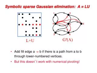
Communication Lower Bound for GE I 0 -B I I 0 -B A I 0 = A I · I A·B 0 0 I 0 0 I I Matrix Multiplication can be “reduced to” GE Not a good way to do matmul but it shows that GE needs at least as much communication as matmul Does GE minimize communication? CS267 Lecture 14
Does GE Minimize Communication? (1/4) for ib = 1 to n-1 step b … Process matrix b columns at a time end = ib + b-1 … Point to end of block of b columns apply BLAS2 version of GEPP to get A(ib:n , ib:end) = P’ * L’ * U’ … let LL denote the strict lower triangular part of A(ib:end , ib:end) + I A(ib:end , end+1:n) = LL-1 * A(ib:end , end+1:n)… update next b rows of U A(end+1:n , end+1:n ) = A(end+1:n , end+1:n ) - A(end+1:n , ib:end) * A(ib:end , end+1:n) … apply delayed updates with single matrix-multiply … with inner dimension b • Model of communication costs with fast memory M • BLAS2 version of GEPP costs • O(n ·b) if panel fits in M: n·b M • O(n · b2) (#flops) if panel does not fit in M: n·b > M • Update of A(end+1:n , end+1:n ) by matmul costs • O( max ( n·b·n / M1/2 , n2 )) • Triangular solve with LL bounded by above term • Total # slow mem refs for GE = (n/b) · sum of above terms CS267 Lecture 14
Does GE Minimize Communication? (2/4) • Model of communication costs with fast memory M • BLAS2 version of GEPP costs • O(n ·b) if panel fits in M: n·b M • O(n · b2) (#flops) if panel does not fit in M: n·b > M • Update of A(end+1:n , end+1:n ) by matmul costs • O( max ( n·b·n / M1/2 , n2 )) • Triangular solve with LL bounded by above term • Total # slow mem refs for GE = (n/b) · sum of above terms • Case 1: M < n (one column too large for fast mem) • Total # slow mem refs for GE = (n/b)*O(max(n b2 , b n2 / M1/2 , n2 )) = O( n2 b , n3/ M1/2 , n3 / b ) • Minimize by choosing b = M1/2 • Get desired lower bound O(n3 / M1/2 ) CS267 Lecture 14
Does GE Minimize Communication? (3/4) • Model of communication costs with fast memory M • BLAS2 version of GEPP costs • O(n ·b) if panel fits in M: n·b M • O(n · b2) (#flops) if panel does not fit in M: n·b > M • Update of A(end+1:n , end+1:n ) by matmul costs • O( max ( n·b·n / M1/2 , n2 )) • Triangular solve with LL bounded by above term • Total # slow mem refs for GE = (n/b) · sum of above terms • Case 2: M2/3 < n M • Total # slow mem refs for GE = (n/b)*O(max(n b2 , b n2 / M1/2 , n2 )) = O( n2 b , n3/ M1/2 , n3 / b ) • Minimize by choosing b = n1/2 (panel does not fit in M) • Get O(n2.5) slow mem refs • Exceeds lower bound O(n3 / M1/2) by factor (M/n)1/2 CS267 Lecture 14
Does GE Minimize Communication? (4/4) • Model of communication costs with fast memory M • BLAS2 version of GEPP costs • O(n ·b) if panel fits in M: n·b M • O(n · b2) (#flops) if panel does not fit in M: n·b > M • Update of A(end+1:n , end+1:n ) by matmul costs • O( max ( n·b·n / M1/2 , n2 )) • Triangular solve with LL bounded by above term • Total # slow mem refs for GE = (n/b) · sum of above terms • Case 3: M1/2 < n M2/3 • Total # slow mem refs for GE = (n/b)*O(max(n b, b n2 / M1/2 , n2 )) = O( n2 , n3/ M1/2 , n3 / b ) • Minimize by choosing b = M/n (panel fits in M) • Get O(n4/M) slow mem refs • Exceeds lower bound O(n3 / M1/2) by factor n/M1/2 • Case 4: n M1/2 – whole matrix fits in fast mem
Alternative cache-oblivious GE formulation (1/2) A = L * U function [L,U] = RLU (A) … assume A is m by n if (n=1) L = A/A(1,1), U = A(1,1) else [L1,U1] = RLU( A(1:m , 1:n/2)) … do left half of A … let L11 denote top n/2 rows of L1 A( 1:n/2 , n/2+1 : n ) = L11-1 * A( 1:n/2 , n/2+1 : n ) … update top n/2 rows of right half of A A( n/2+1: m, n/2+1:n ) = A( n/2+1: m, n/2+1:n ) - A( n/2+1: m, 1:n/2 ) * A( 1:n/2 , n/2+1 : n ) … update rest of right half of A [L2,U2] = RLU( A(n/2+1:m , n/2+1:n) ) … do right half of A return [ L1,[0;L2] ] and [U1,[ A(.,.) ; U2 ] ] • Toledo (1997) • Describe without pivoting for simplicity • “Do left half of matrix, then right half” CS267 Lecture 14
Alternative cache-oblivious GE formulation (2/2) function [L,U] = RLU (A) … assume A is m by n if (n=1) L = A/A(1,1), U = A(1,1) else [L1,U1] = RLU( A(1:m , 1:n/2)) … do left half of A … let L11 denote top n/2 rows of L1 A( 1:n/2 , n/2+1 : n ) = L11-1 * A( 1:n/2 , n/2+1 : n ) … update top n/2 rows of right half of A A( n/2+1: m, n/2+1:n ) = A( n/2+1: m, n/2+1:n ) - A( n/2+1: m, 1:n/2 ) * A( 1:n/2 , n/2+1 : n ) … update rest of right half of A [L2,U2] = RLU( A(n/2+1:m , n/2+1:n) ) … do right half of A return [ L1,[0;L2] ] and [U1,[ A(.,.) ; U2 ] ] • Mem(m,n) = Mem(m,n/2) + O(max(m·n,m·n2/M1/2)) + Mem(m-n/2,n/2) 2 · Mem(m,n/2) + O(max(m·n,m·n2/M1/2)) = O(m·n2/M1/2 + m·n·log M) = O(m·n2/M1/2 ) if M1/2·log M = O(n)
Explicitly Parallelizing Gaussian Elimination • Parallelization steps • Decomposition: identify enough parallel work, but not too much • Assignment: load balance work among threads • Orchestrate: communication and synchronization • Mapping: which processors execute which threads (locality) • Decomposition • In BLAS 2 algorithm nearly each flop in inner loop can be done in parallel, so with n2 processors, need 3n parallel steps, O(n log n) with pivoting • This is too fine-grained, prefer calls to local matmuls instead • Need to use parallel matrix multiplication • Assignment and Mapping • Which processors are responsible for which submatrices? for i = 1 to n-1 A(i+1:n,i) = A(i+1:n,i) / A(i,i) … BLAS 1 (scale a vector) A(i+1:n,i+1:n) = A(i+1:n , i+1:n ) … BLAS 2 (rank-1 update) - A(i+1:n , i) * A(i , i+1:n) CS267 Lecture 14
Different Data Layouts for Parallel GE Bad load balance: P0 idle after first n/4 steps Load balanced, but can’t easily use BLAS2 or BLAS3 1) 1D Column Blocked Layout 2) 1D Column Cyclic Layout Can trade load balance and BLAS2/3 performance by choosing b, but factorization of block column is a bottleneck Complicated addressing, May not want full parallelism In each column, row b 4) Block Skewed Layout 3) 1D Column Block Cyclic Layout Bad load balance: P0 idle after first n/2 steps The winner! 6) 2D Row and Column Block Cyclic Layout 5) 2D Row and Column Blocked Layout CS267 Lecture 14
Distributed GE with a 2D Block Cyclic Layout CS267 Lecture 9
Matrix multiply of green = green - blue * pink CS267 Lecture 9
Review of Parallel MatMul • Want Large Problem Size Per Processor • PDGEMM = PBLAS matrix multiply • Observations: • For fixed N, as P increasesn Mflops increases, but less than 100% efficiency • For fixed P, as N increases, Mflops (efficiency) rises • DGEMM = BLAS routine • for matrix multiply • Maximum speed for PDGEMM • = # Procs * speed of DGEMM • Observations: • Efficiency always at least 48% • For fixed N, as P increases, efficiency drops • For fixed P, as N increases, efficiency increases CS267 Lecture 14
PDGESV = ScaLAPACK Parallel LU • Since it can run no faster than its • inner loop (PDGEMM), we measure: • Efficiency = • Speed(PDGESV)/Speed(PDGEMM) • Observations: • Efficiency well above 50% for large enough problems • For fixed N, as P increases, efficiency decreases (just as for PDGEMM) • For fixed P, as N increases efficiency increases (just as for PDGEMM) • From bottom table, cost of solving • Ax=b about half of matrix multiply for large enough matrices. • From the flop counts we would expect it to be (2*n3)/(2/3*n3) = 3 times faster, but communication makes it a little slower. CS267 Lecture 14
Does ScaLAPACK Minimize Communication? • Lower Bound: O(n2 / P1/2 ) words sent in O(P1/2 ) mess. • Attained by Cannon for matmul • ScaLAPACK: • O(n2 log P / P1/2 ) words sent – close enough • O(n log P ) messages – too large • Why so many? One reduction (costs O(log P)) per column to find maximum pivot • Need to abandon partial pivoting to reduce #messages • Suppose we have n x n matrix on P1/2 x P1/2 processor grid • Goal: For each panel of b columns spread over P1/2 procs, identify b “good” pivot rows in one reduction • Call this factorization TSLU = “Tall Skinny LU” • Several natural bad (numerically unstable) ways explored, but good way exists • SC08, “Communication Avoiding GE”, D., Grigori, Xiang CS267 Lecture 14
Choosing Pivots Rows by “Tournament” W1 W2 W3 W4 W1’ W2’ W3’ W4’ P1·L1·U1 P2·L2·U2 P3·L3·U3 P4·L4·U4 Choose b pivot rows of W1, call them W1’ Choose b pivot rows of W2, call them W2’ Choose b pivot rows of W3, call them W3’ Choose b pivot rows of W4, call them W4’ Wnxb = = Choose b pivot rows, call them W12’ Choose b pivot rows, call them W34’ = P12·L12·U12 P34·L34·U34 = P1234·L1234·U1234 Choose b pivot rows W12’ W34’ Go back to W and use these b pivot rows (move them to top, do LU without pivoting) CS267 Lecture 14
Minimizing Communication in TSLU LU LU LU LU W1 W2 W3 W4 LU Parallel: W = LU LU LU W1 W2 W3 W4 Sequential: LU W = LU LU LU LU W1 W2 W3 W4 LU Dual Core: W = LU LU LU LU Multicore / Multisocket / Multirack / Multisite / Out-of-core: ? Can Choose reduction tree dynamically CS267 Lecture 14
Making TSLU Numerically Stable • Stability Goal: Make ||A – PLU|| very small: O(machine_precision · ||A||) • Details matter • Going up the tree, we could do LU either on original rows of W, or computed rows of U • Only first choice stable • Thm: New scheme as stable as Partial Pivoting (PP) in following sense: get same results as PP applied to different input matrix whose entries are blocks taken from input A • CALU – Communication Avoiding LU for general A • Use TSLU for panel factorizations • Apply to rest of matrix • Cost: redundant panel factorizations (extra O(n2) flops – ok) • Benefit: • Stable in practice, but not same pivot choice as GEPP • One reduction operation per panel: reduces latency to minimum CS267 Lecture 14
Performance vs ScaLAPACK • TSLU • IBM Power 5 • Up to 4.37x faster (16 procs, 1M x 150) • Cray XT4 • Up to 5.52x faster (8 procs, 1M x 150) • CALU • IBM Power 5 • Up to 2.29x faster (64 procs, 1000 x 1000) • Cray XT4 • Up to 1.81x faster (64 procs, 1000 x 1000) • See INRIA Tech Report 6523 (2008), paper at SC08 CS267 Lecture 14
CALU speedup prediction for a Petascale machine - up to 81x faster P = 8192 Petascale machine with 8192 procs, each at 500 GFlops/s, a bandwidth of 4 GB/s.
Which algs for LU (and QR) reach lower bounds? • LU for solving Ax=b, QR for least squares • LAPACK attains neither, depending on relative size of M, n • Recursive sequential algs minimize bandwidth, not latency • Toledo for LU, Elmroth/Gustavson for QR • ScaLAPACK attains bandwidth lower bound • But sends too many messages • New LU and QR algorithms do attain both lower bounds, both sequential and parallel • LU: need to abandon partial pivoting (but still stable) • QR: similar idea of reduction tree as for LU • Neither new alg works for multiple memory hierarchy levels • Open question! • See EECS TR 2008-89 for QR, SC08 paper for LU
Do any Cholesky algs reach lower bounds? • Cholesky factors A = LLT , for Ax=b when A=AT and positive definite • Easier: Like LU, but half the arithmetic and no pivoting • LAPACK (with right block size) or recursive Cholesky minimize bandwidth • Recursive: Ahmed/Pingali, Gustavson/Jonsson, Andersen/ Gustavson/Wasniewski, Simecek/Tvrdik, a la Toledo • LAPACK can minimize latency with blocked data structure • Ahmed/Pingali minimize bandwidth and latency across multiple levels of memory hierarchy • Simultaneously minimize communication between all pairs L1/L2/L3/DRAM/disk/… • “Space-filling curve layout”, “Cache-oblivious” • ScaLAPACK minimizes bandwidth and latency (mod log P) • Need right choice of block size • Details in EECS TR 2009-29 CS267 Lecture 14
Space-Filling Curve Layouts • For both cache hierarchies and parallelism, recursive layouts may be useful • Z-Morton, U-Morton, and X-Morton Layout • Other variations possible • What about the user’s view? • Fortunately, many problems can be solved on a permutation • Never need to actually change the user’s layout CS267 Lecture 14
Summary of dense sequential algorithms attaining communication lower bounds • Algorithms shown minimizing # Messages use (recursive) block layout • Not possible with columnwise or rowwise layouts • Many references (see reports), only some shown, plus ours • Cache-oblivious are underlined, Green are ours, ? is unknown/future work
Summary of dense 2D parallel algorithms attaining communication lower bounds • Assume nxn matrices on P processors, memory per processor = O(n2 / P) • ScaLAPACK assumes best block size b chosen • Many references (see reports), Green are ours • Recall lower bounds: • #words_moved = ( n2 / P1/2 ) and #messages = ( P1/2 )
T T T A A B C C Fork-Join vs. Dynamic Execution on Multicore Source: Jack Dongarra Fork-Join – parallel BLAS Time DAG-based – dynamic scheduling Time saved Experiments on Intel’s Quad Core Clovertown with 2 Sockets w/ 8 Treads 44
Achieving Asynchronicity on Multicore Source: Jack Dongarra • The matrix factorization can be represented as a DAG: • nodes: tasks that operate on “tiles” • edges: dependencies among tasks • Tasks can be scheduled asynchronously and in any order as long as dependencies are not violated. Systems: PLASMA for multicore MAGMA for CPU/GPU CS267 Lecture 14
Intel’s Clovertown Quad Core Source: Jack Dongarra 3 Implementations of LU factorization Quad core w/2 sockets per board, w/ 8 Treads 3. DAG Based (Dynamic Scheduling) 2. ScaLAPACK (Mess Pass using mem copy) 1. LAPACK (BLAS Fork-Join Parallelism) 8 Core Experiments
Dense Linear Algebra on GPUs • Source: Vasily Volkov’s SC08 paper • Best Student Paper Award • New challenges • More complicated memory hierarchy • Not like “L1 inside L2 inside …”, • Need to choose which memory to use carefully • Need to move data manually • GPU does some operations much faster than CPU, but not all • CPU and GPU like different data layouts CS267 Lecture 14
Motivation • NVIDIA released CUBLAS 1.0 in 2007, which is BLAS for GPUs • This enables a straightforward port of LAPACK to GPU • Consider single precision only • Goal: understand bottlenecks in the dense linear algebra kernels • Requires detailed understanding of the GPU architecture • Result 1: New coding recommendations for high performance on GPUs • Result 2: New , fast variants of LU, QR, Cholesky, other routines CS267 Lecture 14
GPU Memory Hierarchy • Register file is the fastest and the largest on-chip memory • Constrained to vector operations only • Shared memory permits indexed and shared access • However, 2-4x smaller and 4x lower bandwidth than registers • Only 1 operand in shared memory is allowed versus 4 register operands • Some instructions run slower if using shared memory CS267 Lecture 14
Memory Latency on GeForce 8800 GTXRepeat k = A[k] where A[k] = (k + stride) mod array_size CS267 Lecture 14
(Some new) NVIDIA coding recommendations • Minimize communication with CPU memory • Keep as much data in registers as possible • Largest, fastest on-GPU memory • Vector-only operations • Use as little shared memory as possible • Smaller, slower than registers; use for communication, sharing only • Speed limit: 66% of peak with one shared mem argument • Use vector length VL=64, not max VL = 512 • Strip mine longer vectors into shorter ones • Final matmul code similar to Cray X1 or IBM 3090 vector codes CS267 Lecture 14