Download
1 / 52
530 likes | 762 Vues
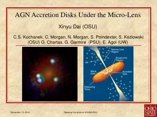
AGN Accretion Disks Under the Micro-Lens X inyu Dai (OSU) C.S. Kochanek, C. Morgan, N. Morgan, S. Poindexter , S. Kozlowski (OSU) G. Chartas , G. Garmire (PSU), E. Agol (UW). Basic Observables. “Einstein Ring” image of quasar host galaxy. Quasar image B. Quasar image D.

E N D
AGN Accretion Disks Under the Micro-Lens Xinyu Dai (OSU) C.S. Kochanek, C. Morgan, N. Morgan, S. Poindexter, S. Kozlowski (OSU) G. Chartas, G. Garmire (PSU), E. Agol (UW) Opening Symposium of KIAA-PKU
Basic Observables “Einstein Ring” image of quasar host galaxy Quasar image B Quasar image D Quasar image A Lens galaxy Quasar image C Hubble Image of Gravitational Lens RXJ1131-1231 (Morgan, Kochanek, Falco, and Dai 2006) Opening Symposium of KIAA-PKU
Intrinsic Variability = Time delays halo structure and distances AB=12.0,AC=9.6, AD=87 days Opening Symposium of KIAA-PKU
Shift To Determine These Delays Opening Symposium of KIAA-PKU
But after shifting and removing the intrinsic source variability, there is still time variability in the flux ratios – Microlensing We observe this in almost all the systems we monitor Opening Symposium of KIAA-PKU
Time Delay in PG1115+080 Measured in X-rays • A1-A2=0.16 days Chartas, Dai, Garmire 2004 Opening Symposium of KIAA-PKU
Applications • Cosmology • Estimates of H0 • CDM Halos Structure • Lensing Statistics • Lens Galaxy • Estimates of Surface Density c • Fraction in stars * • Average stellar mass <M> • ISM Properties • Quasar • Accretion disk structure • Spectral properties using the lensing magnification Opening Symposium of KIAA-PKU
Schematic Plot of a Gravitational Lens Dos Dol Dls Image Source ξ η Opening Symposium of KIAA-PKU
Deflection Potential Analogy to Gravitational Potential Opening Symposium of KIAA-PKU
Relate to Observables (Blandford & Narayan 1986) Geometric Time Delay Gravitational Time Delay (u,v) source position (x,y) image position • Time Delay • Image Position • Magnification (flux) Opening Symposium of KIAA-PKU
Time Delay: Hubble Constant and CDM Halo Structure Time delays measure a combination of H0 and the surface density t 2tisothermal(1<>)/H0 to lowest order Current Direction: Fix H0 and constrain the CDM Halo Structure Kochanek & Schechter 2004 Opening Symposium of KIAA-PKU
What Determines an Image’s Flux? Beyond Source Variability • What contributes to these derivatives? All scales are equally important! • Overall smooth potential – the “macro” model • Satellites/CDM substructure – millilensing • Stars – microlensing • The source size matters because it can average out the smaller scale structures in the magnification pattern • Differential extinction between the images Opening Symposium of KIAA-PKU
Anomalous Flux Ratios: Gravity, ISM or Bad Models? minimum • The close pair images should have similar flux saddle saddle Hubble Image of SDSS0924+0219 minimum Opening Symposium of KIAA-PKU
Dust Extinction Is Observed And you can use it to study dust to z~1 A roughly Galactic extinction curve at z=0.83 (Motta et al 2002) 2175 A feature Opening Symposium of KIAA-PKU
Soft X-ray Absorption is Correlated With Dust and you can use it to study the evolution of the dust to gas ratio Galactic Stars (Bohlin et al 1978) Dai et al. (2006, 2008) Opening Symposium of KIAA-PKU
Anomalies Exist Even for Big Radio Sources “CDM Substructure” Dalal & Kochanek (2002) See also Mao & Schneider (1998); Mao et al. (2004) Springel, White & Tormen (1999) Opening Symposium of KIAA-PKU
But What About Small Substructures (Stars)? Source plane scale=40<E> 2h-1<M/M•>1/2pc=335<M/M•>1/2as B C D A For a 109M• black hole RBH=0.0001pc =0.01as =0.l<M/M•>-1/2pixels Opening Symposium of KIAA-PKU
Length Scales Set by the mass of the lenses and the distances • Lens galaxy M~1010M• E~1arcsec • CDM sub-haloM~106M• E~10 milliarcsec • Star M~M• E~10 microarcsec • Microlensing is not sensitive to large source size, but millilensing do. Opening Symposium of KIAA-PKU
Time Scales set by the crossing time of the Einstein radius • Milli-lensing (by CDM sub-halos) has longer time scale than microlensing (by stars) • ISM in the lens galaxy does not vary on short time scales Opening Symposium of KIAA-PKU
Monitoring Leads to MicrolensingVariability (OGLE light curves of Q2237+030) Opening Symposium of KIAA-PKU
How to use microlensing to measure the source size? — Qualitative Approach • Larger sources smooth the magnification pattern and have smaller microlensing variability. Opening Symposium of KIAA-PKU
Qualitative Approach (Cont’d) • Comparing microlensing variability • IR size > optical size • (Agol et al. 2000) • Optical > X-ray > Iron K Line • (Dai et al. 2003) • Opitcal Narrow line > optical continuum • (Mediavilla et al. 1998) Opening Symposium of KIAA-PKU
Quantitative Approach— Fitting the Microlensing Light Curve Galactic Binary microlensing eventMACHO 98-SMC-1 In this case solutions must include binary orbital motion….. Afonso et al. 2000 Opening Symposium of KIAA-PKU
Let’s Just Do The Same Thing Although a Monte-Carlo Approach in needed Opening Symposium of KIAA-PKU
Let’s Just Do The Same Thing (Cont’d) • We just generate those messy magnification patterns, pick a source size/structure, randomly draw light curves and fit the data • We keep the acceptable solutions • We then calculate the probability distributions for interesting physical variables • We can get light curves that are statistically good fits to the data Opening Symposium of KIAA-PKU
Examples of Magnification Patterns in the Monte-Carlo Simulations Image A (a minimum) */=1 */=0.5 */=0.25 */=0.125 Image C (a saddle point) Opening Symposium of KIAA-PKU
What Matters? • Velocities – sets the time scales – higher velocities give more rapid variability at fixed source size • Mean stellar masses – sets the length scale – higher mean masses give longer time scales at fixed velocity and smaller variability amplitudes at fixed source size • Source size – sets the smoothing – larger sizes give reduced variability amplitudes and longer time scales for fixed mean mass and velocity • Surface density in stars – sets the statistics of the microlensing Opening Symposium of KIAA-PKU
Sometimes, brute force is the solution…. Fits to OGLEI data for Q2237 1 solution in 10^14 trials We used at least 10000 solutions to estimate the interesting parameters Kochanek 2004 Opening Symposium of KIAA-PKU
Finally the Accretion Disk Size • We obtain probability distributions for the disk size. Opening Symposium of KIAA-PKU
Testing the Simplest Accretion Disk Theory Opening Symposium of KIAA-PKU
Beginning to Test Accretion Disk Theory – Size versus Mass Morgan et al. (2007) Black hole masses estimated from emission line-width/mass correlations Opening Symposium of KIAA-PKU
Size versus Wavelength (Temperature) From Microlensing Poindexter et al. 2007 HE1104-1805 A was bright and blue when found, now close to emission line/mid-IR flux ratio and red Opening Symposium of KIAA-PKU
Fit Models With Size Rβ Corresponding To TR-1/β In thin disk theory β=4/3 Consistent with theory but could allow a shallower slope Opening Symposium of KIAA-PKU
X-Ray Emission from AGN • Inverse Compton emission • However, geometric configuration is uncertain Opening Symposium of KIAA-PKU
X-ray Microlensing in Q2237+030 Opening Symposium of KIAA-PKU
Can Also Examine Thermal versus Nonthermal Emission Opening Symposium of KIAA-PKU
X-ray Emission Tracks Inner Disk Edge? X-ray: ~10-20 rg Optical: ~100-200 rg Dai et al. (2008) Opening Symposium of KIAA-PKU
Issues of Observation We monitor ~20 lenses well at at one wavelength (R band), with lesser coverage at J, I, V and B with the SMARTS 1.3m telescope at CTIO, much worse for Northern lenses with the MDM 2.4m – now have ~(4 years)(20 lenses)(3 images) = 2.4 image monitoring centuries UV monitoring with HST for two lenses (RXJ1131 and Q2237) – fortunately with ACS semi-death both of these lenses have flux past their Lyman limits and can be observed with the ACS/SBC! X-ray monitoring with Chandra for RXJ1131 and Q2237 sparse coverage of other lenses from archive and other programs Increase the sample size to ~10 monitored with HST and Chandra The challenge problem – microlensing of the Iron K line – hints in published data (Dai and Chartas), but quantitative results for the size of the K emission region are a Megasecond CXO project Opening Symposium of KIAA-PKU
Summary • Microlensing is the first new probe of accretion disk structure in ~10 years • Disk sizes scale with black hole mass as in thin disk theory M2/3 • The absolute size is roughly consistent with theory but larger than expected for black body radiation and the TR-3/4 • The scaling of disk size with wavelength is consistent with this temperature profile but could allow a flatter profile that would help to solve the size problem • X-ray emission is more compact and seems to trace the scale of the inner disk edge • We are primarily data limited at the present time given the ability to collect the necessary data, we can dramatically improve over our existing results Opening Symposium of KIAA-PKU
For Quasar Accretion Disks We Want to Understand the Size Should be able to study structure of quasar accretion disks because variability amplitude source size Opening Symposium of KIAA-PKU
Scales as expected with Black Hole MassRM2/3 The implied efficiency is somewhat low or the MBH are systematically high Opening Symposium of KIAA-PKU
Amplitude Does Depend on Wavelength Opening Symposium of KIAA-PKU
Radio Data Shows No Absorption Despite seeing some scatter broadened images No sign of the frequency dependence we would expect for a propagation effect – consider an optical depth =5(/5GHz) Opening Symposium of KIAA-PKU
Problems In the Mass Models? (Kochanek & Dalal, Yoo et al., Congdon & Keeton) • Lens models for 2/4 image lenses are underconstrained if you allow arbitrary angular structure • Lenses with additional images or Einstein rings require models that are consistent with ellipsoids B1933+503 Opening Symposium of KIAA-PKU
Oversimplified Disk Model? Why are the microlensing sizes large – use fancier disk models to try to simultaneously fit flux, spectrum and microlensing sizes based on more realistic Hubeny et al disk models – basic problem remains – disks too big for their flux (also a problem for Galactic systems like CVs). Opening Symposium of KIAA-PKU
Contamination of the Continuum? • We are “assuming” that we are monitoring continuum emission from the quasar accretion disk – what if the “continuum” emission is not? • Contamination from obvious broad lines – line emission is really on much bigger (and less microlensed, but not unmicrolensed – e.g. Richards et al) scales • Contamination from the pseudo-continuum – Iron lines and Balmer continuum emission • Testing for this, but so far, the answer is that this does not change the results… Opening Symposium of KIAA-PKU
Issues of Observation Given an infinitely long light curve, you should be able to reconstruct all lens properties aside from the Einstein units conversion – but how close to “infinite”? Very crudely, you have to monitor an image for an Einstein time to start getting a “fair” sample of the microlensing for that image (~15 years) – at this point you will start sampling the pattern – for a single lens (2 or 4 images) you need 15/(2 or 4) 4-7 years The metric for a microlensing program is “image monitoring years” and you want to get to several image monitoring centuries Opening Symposium of KIAA-PKU
The Flux Size Problem (Pooley et al originally) These “flux sizes” are systematically smaller than either the microlensing or the thin disk theory sizes – not thermally radiating or flatter temperature profiles Opening Symposium of KIAA-PKU
Issues of Computation • This is a tough problem – picking light curves at random from these patterns and fitting them to actual data is not easy – it probably becomes exponentially harder as the light curve length increases… • But, that’s not the big problem – the exponential is still small (except for Q2237). • The big problem is that the stars move – the patterns are animated, not static! • Probably matters most for mass estimates • Broadens errors for other variables, but who wants exaggerated error bars? • Huge computational challenge – we have to use 81922 magnification patterns for many/most problems at a cost of 256 MByte/image and source size and for many problems we should be using 162842 patterns. Animating a pattern requires ~100 such patterns 25 GBytes/image and source size even for the 81922 patterns Opening Symposium of KIAA-PKU
Are Galaxies Composed of Stars? RXJ1131-1231 Q2237+0305 Most lenses, like RXJ1131-1231, should only have a small fraction of the surface density near the quasar images comprised of stars (/*~0.1 to 0.2), but one lens, Q2237+0305, where we see the images through the bulge of a low redshift spiral galaxy, should be almost all stars (/*~1) Opening Symposium of KIAA-PKU