Download
1 / 8
80 likes | 241 Vues
Characteristics of Precipitation Features in the Central Andes Karen Mohr 1 , Daniel Slayback 2 , and Karina Yager 2 1 Code 610, NASA GSFC; 2 Code 618, NASA GSFC and SSAI, Inc.

E N D
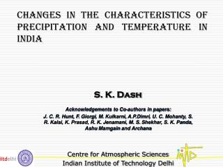
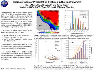
Characteristics of Precipitation Features in the Central Andes Karen Mohr1, Daniel Slayback2, and Karina Yager2 1Code 610, NASA GSFC; 2Code 618, NASA GSFC and SSAI, Inc. • Climatologically, the Central Andes range from 7°S to 21°S, covering southern Peru, Bolivia, and northern Chile, and containing 90% of the world’s tropical glaciers. We used TRMM-observed precipitation features (PF) and surface observations to learn more about the spectra of PF size, intensity, and rainfall rates of observed PFs (1998-2012) in the Andean highlands (> 1000 m). • The majority of annual rainfall in the Central Andes is contributed by PFs with • Weak, shallow (< 12 km) convection, • Short durations (< 60 min), • Light to light-moderate rainfall rates (0.5-4.0 mm hr-1). • Well-organized and intense PFs do occur but there are not enough of them to make an impact on regional rainfall statistics. • The Central Andes PFs tended to be smaller and weaker than PFs in comparably dry (West Africa), mountainous (Himalayas), and dynamically linked (Amazon) regions in the tropics. (1b) (1a) Figure 1:(a) Area map of mean annual rainfall (1998-2012). The white contour is the 1000 m elevation line defining the eastern and western boundaries of the study area. (b) TRMM-observed PF rain rates vs. annual rainfall contribution for arid (blue), humid (red), and transitional (green) climate zones. (2b) (2a) Figure 2: (a) Rain gauge data from Tuni, Bolivia (16.67°S, 68.13°W, T on Fig. 1a) showing the duration vs. rain rate for events during the wet season Nov 2011-Apr 2012. (b) PF echo height vs. annual rainfall contribution (bars) and cumulative total (lines) for Central Andes (orange) and for West Africa (purple). Earth Sciences Division - Atmospheres
Name: Karen Mohr, NASA GSFC, Code 610 E-mail: karen.mohr-1@nasa.gov Phone: 301-614-6360 References: Mohr, K. I., D. Slayback, K. Yager, 2014: Characteristics of precipitation features and annual rainfall during the TRMM era in the Central Andes. Journal of Climate, in press, doi: http://dx.doi.org/10.1175/JCLI-D-13-00592.1. Data Sources: Gridded monthly multi-satellite rainfall product (TRMM 3B43); TRMM Precipitation Features (PF) database from the University of Utah, a “value added” product derived from Level 1 observations that defines PFs as contiguous raining PR and TMI pixels. Surface observations from our own sites in Bolivia at Tuni and Sajama (8.11°S, 68.89°W, “S” in Fig. 1a) and historical data from local collaborators in Bolivia and Peru. We are grateful for support for this work from G. Gutman, program manager for LC/LUC. Technical Description of Figures: Figure 1: (a) The mean annual rainfall (mm) from the 3B43 product (1998-2012). The levels are multiples of 180 mm based on the GIS-derived breakpoints in the regional rainfall total histogram. The “T” and “S” illustrate the differences in annual totals between Tuni and Sajama despite similar altitudes. The white contour highlights the 1000-m elevation line. The legend colors and the breakpoints at 720 mm and 1440 mm distinguish between arid (gray to blue), transitional (green to orange), and humid (red to brown) climate zones with similar seasonality but different diurnal cycles and rainfall rate histograms. Note a generally east to west decrease in rainfall, modified by elevation (e.g., southeastern Peru). (b) Rainfall rate histograms for the three climate zones shift to higher values from arid (blue) to humid (red). From 0.5−4 mm hr-1 is 90% of arid (blue), 75% of transitional (green), 60% of humid (red) total rainfall. Despite some differences in their histograms, all three climate zones in the Central Andes demonstrate a similar dependence on light rainfall events for their annual total rainfall. Figure 2: (a) A scatter diagram (event average rain rate versus duration) for rainfall events observed by our tipping bucket rain gauge at Tuni. Each month is indicated by a different shape and color marker, but there are no significant monthly differences. 50% or more of events are < 60 min and < 3 mm hr-1 and 90% are < 120 min and < 6 mm hr-1. (b) PF maximum echo height (km) vs. contribution to annual rainfall [total (bars) and cumulative (lines)] for the Central Andes (orange) and a similarly dry region, West Africa (purple). The majority of rainfall in the Central Andes is from shallow convection (≤ 12 km) compared to deep convection in West Africa (≥ 16 km). Compared to West Africa and other tropical regions, rainfall events in the Central Andes tend to be lighter (< 6 mm hr-1) and largely from shallow, weak convection. Scientific significance: This project was part of a larger multi-disciplinary study, “The Impact of Disappearing Tropical Andean Glaciers on Pastoral Agriculture” (PI Dan Slayback). Threats to ancient rangelands in the high Andes due to glacier recession and climate change inspired our work to characterize the glacier recession rates, valley hydrology and ecosystem functioning, and regional rainfall regimes from field and remote sensing data. We provide strong evidence than rangeland health is closely tied to the light, frequent rainfall events that occur in the present climate and continue to work toward understanding how these rainfall regimes will change in the future using regional climate modeling. Relevance for Future Missions: This project is directly relevant to studying NASA goals of understanding climate change impacts, present and future, using land imaging and atmospheric remote sensing data products from multiple current and historic missions (LandSat, TRMM, Aqua/Terra) for analysis and model validation. Our work is directly relevant to pre-Decadal Survey discussions about the needs for future instruments that can continue the historical record of land cover and precipitation. Earth Sciences Division - Atmospheres
Wind Retrieval Algorithms for the HIWRAP Airborne Doppler Radar with Applications to Hurricanes during GRIPStephen Guimond, Code 612, NASA GSFC and UMD/ESSIC • Knowledge of the three-dimensional (3D) distribution of winds in precipitating systems such as hurricanes is crucial for understanding their dynamics and predicting their evolution. The present work develops a mathematical/computational technique for retrieving 3D winds from a new class of airborne Doppler radar that scans in a cone below the aircraft. • The focus is on NASA/GSFC’s new High-altitude Imaging Wind and Rain Airborne Profiler (HIWRAP) flying on the NASA Global Hawk aircraft. • New wind retrieval algorithms are developed that can provide the three Cartesian velocity components over the entire radar sampling volume at high resolution. • Using a 3D variational solution method, the horizontal winds have an accuracy of ~ 1.5 – 2.0 m s-1 with a ~ 1.5 m s-1 error for vertical winds. • HIWRAP wind retrievals reveal an undetected circulation center in Tropical Storm Matthew and the detailed structure of rapidly intensifying Hurricane Karl during the NASA GRIP field experiment conducted in 2010. (a) (b) (c) (d) Figure 1:(a) shows the scanning geometry of HIWRAP. (b) shows HIWRAP wind vector retrievals at 2 km height in Hurricane Karl (2010) using a synthesis of ~ 12 h of data. (c) shows a GOES IR image of Tropical Storm Matthew (2010) overlaid with the Global Hawk track. (d) shows HIWRAP wind vector retrievals at 3 km height along the blue flight segments shown in the GOES image of Matthew. Additional details are described on page 2. Earth Sciences Division - Atmospheres
Name: Stephen Guimond, NASA GSFC, Code 612 and UMD/ESSIC E-mail: stephen.guimond@nasa.gov Phone: 301-614-5809 Reference: Guimond, S.R., L. Tian, G.M. Heymsfieldand S.J. Frasier, 2014: Wind retrieval algorithms for the IWRAP and HIWRAP airborne Doppler radars with applications to hurricanes. Journal of Atmospheric and Oceanic Technology, in press. doi: http://dx.doi.org/10.1175/JTECH-D-13-00140.1 Contributors: Lin Tian (NASA/GSFC and MSU), Gerald M. Heymsfield (NASA/GSFC), Matt McLinden (NASA/GSFC) and Lihua Li (NASA/GSFC). Data Sources: NASA/GSFC HIWRAP airborne Doppler radar, GOES IR data. Technical Description of Figures: Figure 1: Panel (a) shows the scanning geometry of HIWRAP flying on the NASA Global Hawk aircraft (altitudes of 18 – 20 km). HIWRAP scans at 16 rpm below the aircraft with a ~ 600 m sampling interval. HIWRAP has two beams (30°and 40° incidence) each at Ku and Ka band. Panel (b) shows HIWRAP horizontal wind vector retrievals overlaid on Ku band reflectivity at 2 km height in Hurricane Karl during the Genesis and Rapid Intensification Processes (GRIP) field experiment conducted in 2010. This figure combines ~ 12 h of data and the grid spacing of the retrievals is 1 km. Panel (c) shows a GOES IR image of the development of Tropical Storm Matthew, also sampled during GRIP. The black lines show the track of the Global Hawk with the blue lines highlighting interesting portions of the storm. The “O” and “X” are the storm center estimates defined by the National Hurricane Center (NHC) and HIWRAP wind retrievals, respectively. Panel (d) figure shows HIWRAP wind vector retrievals at 3 km height along the blue lines in the IR image of Matthew. The “O” and “X” are the same as in panel (c). The HIWRAP retrievals show that the NHC center position is likely erroneous and highlights the critical importance of both the Global Hawk and the HIWRAP radar for tropical cyclone monitoring and research. Scientific significance: Atmospheric winds in precipitating systems are one of the most fundamental quantities of the atmosphere and are crucial for understanding and forecasting high impact events such as hurricanes. The algorithms described in this paper will allow retrievals of three-dimensional winds at high resolution from a new class of airborne radar that fly on the unmanned Global Hawk aircraft. The new algorithms, radar and aircraft will allow the potential for significant improvements in our understanding and monitoring of ocean based precipitating systems. Relevance for future science and relationship to Decadal Survey: The retrieval of three-dimensional atmospheric winds from space-based instruments has never been done before, and the HIWRAP radar along with the present retrieval algorithms can provide a testing ground for future space instrumentsand scientific understanding. Earth Sciences Division - Atmospheres
Detection of mountain lee waves in MODIS NIR column water vapor A. Lyapustin, M. J. Alexander, L. Ott, A. Molod, Y. Wang, B. Holben, J. Susskind Code 613, NASA GSFC; NWRA-CoRA Office; UMCP; UMBC Mountain gravity (lee) waves are caused by an air flow over mountain ridges within a stably stratified atmosphere. Breaking waves and small-scale waves can be a source of turbulence and strong vertical air currents, which can be an aviation hazard. Atmos-pheric gravity waves have been widely studied using high-resolution temperature observations from space [e.g., Alexander & Teitelbaum, 2011] . Mountain-generated waves have been observed using the MODIS 6.7μm channel which has peak sensitivity at altitudes ~550hPa. Using the MAIAC algorithm [Lyapustin et al., 2011], we have discovered mountain lee waves in the total column water vapor (CWV) derived from MODIS near-IR measurements (0.94m). Figure 1 shows two examples of lee waves in the CWV product, which are frequently observed east of the Appalachian range during the fall-spring period and on summer days with low to moderate humidity. On such days, the air of a dry colder upper layer is alternately lifted and lowered by gravity waves, causing convergence and diver-gence of air in the moist bottom layer, which is seen as bands in the CWV field. Since the bulk of CWV is confined to the boundary layer, these may be the lowest level signatures of mountain waves presently detected by remote sensing over the land [Lyapustin et al., 2014]. This result is supported by radiosonde and atmospheric stability analysis based on GEOS-5 meteorological fields. The observed phenomenon has relevance to modeling of the boundary layer atmospheric dynamics, correction of repeat-pass Interferometric Synthetic Aperture Radar data, retrievals of green-house gases (e.g., CO2 and CH4) and other applications. Figure 1 (Top):MODIS Terra NIR Column Water Vapor (CWV) image reveals gravity waves from Appalachian Mountains in the mid-Atlantic USA region on June 2, 2011. The inset shows radiosonde (black and blue) and GEOS-5 (red) derived profiles of the Scorer Parameter (SP), related to atmospheric stability, at Dulles Airport. The trapped waves exist at altitudes from ~1km to 2km where SP exceeds horizontal wavenumber of the CWV waves (dashed line). The MODIS Terra RGB image is shown on the left. (Bottom) Example of gravity waves from MODIS Aqua data on March 18, 2011. Earth Sciences Division - Atmospheres 0 1.0 2.0 3.0 4.0 cm
Name: Alexei Lyapustin, NASA GSFC Code 613E-mail: Alexei.I.Lyapustin@nasa.govPhone: 301-614-5998 References: Alexander, M. J., and H. Teitelbaum (2011), Three-dimensional properties of Andes mountain waves observed by satellite: A case study, J. Geophys. Res., 116, D23110, doi:10.1029/2011JD016151. Lyapustin, A., Y. Wang, I. Laszlo, R. Kahn, S. Korkin, L. Remer, R. Levy, and J. S. Reid (2011), Multi-angle Implementation of Atmospheric Correction (MAIAC): 2. Aerosol algorithm, J. Geophys. Res., 116, D03211, doi:10.1029/2010JD014986. Lyapustin, A., M. J. Alexander, L. Ott, A. Molod, B. Holben, J. Susskind, and Y. Wang (2014), Observation of mountain lee waves with MODIS NIR column water vapor, Geophys. Res. Lett., 41, doi:10.1002/2013GL058770. Data Sources: MODIS Terra and Aqua Level 1B data; GEOS-5. Technical Description of Figures: Figure 1 (Top):MODIS Terra NIR Column Water Vapor (CWV) image reveals gravity waves from Appalachian Mountains in the mid-Atlantic USA region on June 2, 2011. The inset shows radiosonde (black and blue) and GEOS-5 (red) derived profiles of the Scorer Parameter (SP), related to atmospheric stability, at Dulles Airport. The trapped waves exist at altitudes from ~1km to 2km where SP exceeds horizontal wavenumber of the CWV waves (dashed line). The MODIS Terra RGB image is shown on the left. (Bottom) Example of gravity waves from MODIS Aqua data on March 18, 2011. Scientific significance: Mountain waves are detected in the MODIS NIR column water vapor. We observe 3-4 to 15 km lee waves with an amplitude of 50-70% of the total CWV. The result is supported by radiosonde and atmospheric stability analysis based on GEOS-5 meteorological fields. In contrast to previous studies based on sounding data which reported gravity waves at altitudes of the midtroposphere and stratosphere, the CWV shows perhaps the lowest near-surface waves (~1-3 km above the surface) that can be detected from remote sensing data over land. Relevance for future science and NASA missions: Water vapor is a potent greenhouse gas. It is a major component of the Earth energy and water cycles and a major parameter in weather forecasting and climate modeling. Accurate knowledge of atmospheric water vapor is crucial to correct the time delay and phase distortions for the repeat-pass Interferometric Synthetic Aperture Radar applications. Lyapustin et al. (2014) showed that MAIAC improves the accuracy of CWV by removing the high (“wet”) bias of MODIS operational CWV product MOD05. Knowledge of variability in CWV at scales ~1km derived from MODIS measurements over land will inform regional and global models of moist processes, which rely on assumptions about the subgrid variability of total water. Remote sensing measurements of greenhouse gases, such as CO2 and CH4, will also benefit from improved characterization of CWV variability because such information allows for more accurate representation of the line broadening by water vapor and potential error reduction. Earth Sciences Division - Atmospheres
The quasi-biennial oscillation is disrupted by geoengineering aerosols V. Aquila1,2, C. I. Garfinkel3, P. A. Newman1, L. D. Oman1, D. W. Waugh2 1Code 614, NASA GSFC, 2GESTAR/Johns Hopkins University, 3Hebrew University Regular West QBO The quasi-biennial oscillation (QBO) is a phenomenon whereby stratospheric tropical zonal winds switch from westerly to easterly with a period of about two years. The QBO affects temperatures and transport of air into and out of the tropics, and is the main source of variability in the tropical stratosphere. Geoengineering is the deliberate modification of the Earth’s climate to counteract global warming. One method recreates the cooling effect of large volcanic eruptions by continuous injection of sulfate aerosol particles into the stratosphere. We quantified the effects of this geoengineering method by simulating different sulfate injections into the Goddard Earth Observing System chemistry-climate model. Injected sulfate aerosols warm the lower stratosphere, prolonging the phase of westerly winds. High sulfate aerosol burdens completely eliminate the wind oscillation. The QBO impacts the composition of the troposphere and stratosphere, monsoon precipitation and the polar vortex strength. Hence, a QBO disruption would have effects well beyond the tropical stratosphere. Extended West QBO No QBO Easterlies Westerlies Figure 1: Here we show the simulated vertical profiles of equatorial stratospheric zonal winds from the start of the geoengineering injection in January 2020 to December 2040. Red shaded areas mark westerly (or eastward blowing) winds, blue shaded areas easterly (or westward blowing) winds. The upper panel shows the control simulation – with no sulfate aerosol. The middle and lower panels show the simulations with geoengineering sulfate burdens of 3.1 Tg-Sulfate (middle) and 4.7 Tg-Sulfate (bottom). Earth Sciences Division - Atmospheres
Name: Valentina Aquila, NASA GSFC, Code 614 E-mail: valentina.aquila@nasa.gov Phone: 301-614-6927 References: Aquila, V., C. I. Garfinkel, P. A. Newman, L. D. Oman, D. W. Waugh, Modifications of the quasi-biennial oscillation by a geoengineering perturbation of the stratospheric aerosol layer. Accepted for publication in Geophysical Research Letters. Data Sources: Future climate simulations performed with the NASA Goddard Earth Observing System, Version 5, Chemistry Climate Model (GEOSCCM). The model simulations are performed using an horizontal resolution of 2.0˚ latitude by 2.5˚ longitude, with 72 vertical hybrid levels from surface to 0.01 hPa. The model is prescribed with sea surface temperatures and sea ice concentrations calculated with the Community Earth System Model (CESM), using emission inventories valid for the Representative Concentration Pathway (RCP) 4.5. Technical Description of Figures: Figure 1: Vertical profiles of the zonal winds, averaged between 2˚S and 2˚N. The geoengineering aerosol is introduced in the simulation by continuously injecting 5 Tg SO2/year at on the Equator at 0˚ longitude between 16km-25km (middle panel) and 22km-25km (lower panel) altitude. GEOSCCM calculates the transformation of SO2 into sulfate aerosol. The higher injection height leads to a larger aerosol equilibrium burden. Scientific significance: Geoengineering is currently being discussed among scientists and policy makers as a last resort to counteract the global warming due to increasing greenhouse gases. Geoengineering, however, would have several effects besides decreasing global temperatures, including stratospheric ozone depletion, change of the water cycle, and regional effects. In this study we show how the stratospheric warming due to the absorption of largely longwave radiation by the aerosol particles would increase the stratospheric vertical residual velocities and strengthen the westerly winds, dramatically changing the stratospheric dynamics and possibly disrupting the QBO. Relevance for future science and relationship to Decadal Survey: Our study shows that a perturbation of the stratospheric aerosol might significantly affect the stratospheric dynamics through heating-induced effects. Recent observations have reported an increase of the stratospheric aerosol burden, mainly due to small volcanic eruptions, but also to a smaller extent to increasing tropospheric emissions transported to the stratosphere through the Asian monsoon convective system. This increase might lead to a change in the background state, and, hence, in the effects of geoengineering. Long-term observations of the stratospheric aerosol layer, such as the ones provided by the NPP-Suomi satellite, are required to gain knowledge of the stratospheric background aerosol and its importance in the climate system. Earth Sciences Division - Atmospheres