Ensemble Learning
Ensemble Learning. CS 6243 Machine Learning Modified from the slides by Dr. Raymond J. Mooney http://www.cs.utexas.edu/~mooney/cs391L And by Dr. Carla P. Gomes http://www.cs.cornell.edu/Courses/cs4700/2008fa/. Ensemble Learning.

Ensemble Learning
E N D
Presentation Transcript
Ensemble Learning CS 6243 Machine Learning Modified from the slides by Dr. Raymond J. Mooney http://www.cs.utexas.edu/~mooney/cs391L And by Dr. Carla P. Gomeshttp://www.cs.cornell.edu/Courses/cs4700/2008fa/
Ensemble Learning • So far – learning methods that learn a single hypothesis, chosen form a hypothesis space that is used to make predictions. • Ensemble learning select a collection (ensemble) of hypotheses and combine their predictions. • Example 1 - generate 100 different decision trees from the same or different training set and have them vote on the best classification for a new example. • Key motivation: reduce the error rate. Hope is that it will become much more unlikely that the ensemble of will misclassify an example.
Training Data Data1 Data m Data2 Learner m Learner2 Learner1 Model1 Model2 Final Model Model m Model Combiner Learning Ensembles • Learn multiple alternative definitions of a concept using different training data or different learning algorithms. • Combine decisions of multiple definitions, e.g. using weighted voting. Source: Ray Mooney
Value of Ensembles • “No Free Lunch” Theorem • No single algorithm wins all the time! • When combing multiple independent and diverse decisions each of which is at least more accurate than random guessing, random errors cancel each other out, correct decisions are reinforced. Source: Ray Mooney
X X X X X X X X X X X X X Example: Weather Forecast
Majority vote Suppose we have 5 completely independent classifiers… If accuracy is 70% for each (.75)+5(.74)(.3)+ 10 (.73)(.32) 83.7% majority vote accuracy 101 such classifiers 99.9% majority vote accuracy Intuitions Note: Binomial Distribution: The probability of observing x heads in a sample of n independent coin tosses, where in each toss the probability of heads is p, is
Ensemble Learning • Another way of thinking about ensemble learning: • way of enlarging the hypothesis space, i.e., the ensemble itself is a hypothesis and the new hypothesis space is the set of all possible ensembles constructible form hypotheses of the original space. Increasing power of ensemble learning: Three linear threshold hypothesis (positive examples on the non-shaded side); Ensemble classifies as positive any example classified positively be all three. The resulting triangular region hypothesis is not expressible in the original hypothesis space.
Different types of ensemble learning • Different learning algorithms • Algorithms with different choice for parameters • Data set with different features (e.g. random subspace) • Data set = different subsets (e.g. bagging, boosting)
Different types of ensemble learning (1) • Different algorithms, same set of training data A1 C1 Training Set L A2 C2 … … An Cn • A: algorithm I; C: classifier
Different types of ensemble learning (2) • Same algorithm, different parameter settings C1 P1 Training Set L P2 A C2 Pn … Cn • P: parameters for the learning algorithm
Different types of ensemble learning (3) • Same algorithm, different versions of data set, e.g. • Bagging: resample training data • Boosting: Reweight training data • Decorate: Add additional artificial training data • RandomSubSpace (random forest): random subsets of features L1 C1 Training Set L L2 A C2 … … Ln Cn In WEKA, these are called meta-learners, they take a learning algorithm as an argument (base learner) and create a new learning algorithm.
Combining an ensemble of classifiers (1) • Voting: • Classifiers are combined in a static way • Each base-level classifier gives a (weighted) vote for its prediction • Plurality vote: each base-classifier predict a class • Class distribution vote: each predict a probability distribution • pC(x) = ΣCCpC(x) / | C |
Combining an ensemble of classifiers (2) • Stacking: a stack of classifiers • Classifiers are combined in a dynamically • A machine learning method is used to learn how to combine the prediction of the base-level classifiers. • Top level classifier is used to obtain the final prediction from the predictions of the base-level classifiers
Combining an ensemble of classifiers (3) • Cascading: • Combine classifiers iteratively. • At each iteration, training data set is extended with the prediction obtained in the previous iteration
Bagging • Create ensembles by “bootstrap aggregation”, i.e., repeatedly randomly resampling the training data (Brieman, 1996). • Bootstrap: draw N items from X with replacement • Each bootstrap sample will on average contain 63.2% of the unique training examples, the rest are replicates. • Bagging • Train M learners on M bootstrap samples • Combine outputs by voting (e.g., majority vote) • Decreases error by decreasing the variance in the results due to unstable learners, algorithms (like decision trees and neural networks) whose output can change dramatically when the training data is slightly changed.
Bagging - Aggregate Bootstrapping • Given a standard training set D of size n • For i = 1 .. M • Draw a sample of size n* n from D uniformly and with replacement • Learn classifier Ci • Final classifier is a vote of C1 .. CM
Boosting • Originally developed by computational learning theorists to guarantee performance improvements on fitting training data for a weak learner that only needs to generate a hypothesis with a training accuracy greater than 0.5 (Schapire, 1990). • Revised to be a practical algorithm, AdaBoost, for building ensembles that empirically improves generalization performance (Freund & Shapire, 1996). • Key Insights: • Instead of sampling (as in bagging) re-weigh examples! • Examples are given weights. At each iteration, a new hypothesis is learned (weak learner) and the examples are reweighted to focus the system on examples that the most recently learned classifier got wrong. • Final classification based on weighted vote of weak classifiers
Construct Weak Classifiers • Using Different Data Distribution • Start with uniform weighting • During each step of learning • Increase weights of the examples which are not correctly learned by the weak learner • Decrease weights of the examples which are correctly learned by the weak learner • Idea • Focus on difficult examples which are not correctly classified in the previous steps • Intuitive justification: models should be experts that complement each other
Combine Weak Classifiers • Weighted Voting • Construct strong classifier by weighted voting of the weak classifiers • Idea • Better weak classifier gets a larger weight • Iteratively add weak classifiers • Increase accuracy of the combined classifier through minimization of a cost function
Adaptive Boosting • Each rectangle corresponds to an example, • with weight proportional to its height. • Crosses correspond to misclassified examples. • Size of decision tree indicates the weight of that hypothesis in the final ensemble.
AdaBoost Pseudocode TrainAdaBoost(D, BaseLearn) For each example di in D let its weight wi=1/|D| Let H be an empty set of hypotheses For t from 1 to T do: Learn a hypothesis, ht, from the weighted examples: ht=BaseLearn(D) Add ht to H Calculate the error, εt, of the hypothesis ht as the total sum weight of the examples that it classifies incorrectly. If εt> 0.5 then exit loop, else continue. Let βt = εt / (1 – εt ) Multiply the weights of the examples that ht classifies correctly by βt Rescale the weights of all of the examples so the total sum weight remains 1. Return H TestAdaBoost(ex, H) Let each hypothesis, ht, in H vote for ex’s classification with weight log(1/ βt ) Return the class with the highest weighted vote total.
Learning with Weighted Examples • Generic approach: replicate examples in the training set proportional to weights (e.g. 10 replicates of an example with a weight of 0.01 and 100 for one with weight 0.1). • Most algorithms can be enhanced to efficiently incorporate weights directly in the learning algorithm • For decision trees, for calculating information gain, when counting example i, simply increment the corresponding count by wi rather than by 1. • Can apply boosting without weights • resample with probability determined by weights • disadvantage: not all instances are used • advantage: if error > 0.5, can resample again
Restaurant Data Decision stump: decision trees with just one test at the root.
Experimental Results on Ensembles(Freund & Schapire, 1996; Quinlan, 1996) • Ensembles have been used to improve generalization accuracy on a wide variety of problems. • On average, Boosting provides a larger increase in accuracy than Bagging. • Boosting on rare occasions can degrade accuracy. • Bagging more consistently provides a modest improvement. • Boosting is particularly subject to over-fitting when there is significant noise in the training data. • Bagging is easily parallelized, Boosting is not.
Random Forest • Leo Breiman, Random Forests, Machine Learning, 45, 5-32, 2001 • Motivation: reduce error correlation between classifiers • Main idea: build a larger number of un-pruned decision trees • Key: using a random selection of features to split on at each node
How Random Forest Work Each tree is grown on a bootstrap sample of the training set of N cases. A number m is specified much smaller than the total number of variables M (e.g. m = sqrt(M)). At each node, m variables are selected at random out of the M. The split used is the best split on these m variables. Final classification is done by majority vote across trees. Source: Brieman and Cutler 27
Advantages of random forest • Error rates compare favorably to Adaboost • More robust with respect to noise. • More efficient on large data • Provides an estimation of the importance of features in determining classification • More info at: http://stat-www.berkeley.edu/users/breiman/RandomForests/cc_home.htm
DECORATE(Melville & Mooney, 2003) • Change training data by adding new artificial training examples that encourage diversity in the resulting ensemble. • Improves accuracy when the training set is small, and therefore resampling and reweighting the training set has limited ability to generate diverse alternative hypotheses.
C1 + + - + - Overview of DECORATE Current Ensemble Training Examples + - - + + Base Learner Artificial Examples
C2 - + - - + - - - + + Overview of DECORATE Current Ensemble Training Examples + C1 - - + + Base Learner Artificial Examples
C3 Overview of DECORATE Current Ensemble Training Examples + C1 - - + + Base Learner C2 - + + + - Artificial Examples
Ensembles and Active Learning • Ensembles can be used to actively select good new training examples. • Select the unlabeled example that causes the most disagreement amongst the members of the ensemble. • Applicable to any ensemble method: • QueryByBagging • QueryByBoosting • ActiveDECORATE
+ + - + - + + - + Active-DECORATE Unlabeled Examples Utility = 0.1 Current Ensemble Training Examples C1 C2 DECORATE C3 C4
0.3 0.2 0.5 + + - + - + - - + - Acquire Label Active-DECORATE Unlabeled Examples Utility = 0.1 0.9 Current Ensemble Training Examples C1 C2 DECORATE C3 C4
Meta decision trees (MDT) • Combining Classifiers with Meta Decision Trees, Ljupco Todorovski and Saso Dzeroski, Machine Learning, 50, 223-249, 2003 • A type of stacking, usually uses different algorithms for different base-level classifiers • A MDT is a decision tree whose leaf leads to a prediction of which base-level classifier should be used • Meta-level attributes could be something calculated from the prediction of the base-level classifiers, or could be just the set of base-level attributes. • Useful when data include instances from heterogeneous sub-domains
Stacking with MDT vs. ODT pC1 1 Conf1 0 conf1 conf1 <= 0.625 > 0.625 <= 0.625 > 0.625 <= 0.625 > 0.625 C2 C1 pC2 pC2 0 1 0 0 1 1 (a) Stacking of C1 and C2 with MDT 0 1 0 1 (b) Stacking of C1 and C2 with ODT • ODT uses class values predicted by base-level classifiers as attributes. (e.g., the test pc1 = 0), while this is not used by MDT • ODT predicts the class value in its leaf nodes, while MDT predicts the base-level classifiers to be used
Netflix Users rate movies (1,2,3,4,5 stars); Netflix makes suggestions to users based on previous rated movies.
http://www.netflixprize.com/index Since October 2006 “The Netflix Prize seeks to substantially improve the accuracy of predictions about how much someone is going to love a movie based on their movie preferences. Improve it enough and you win one (or more) Prizes. Winning the Netflix Prize improves our ability to connect people to the movies they love.”
Supervised learning task Training data is a set of users and ratings (1,2,3,4,5 stars) those users have given to movies. Construct a classifier that given a user and an unrated movie, correctly classifies that movie as either 1, 2, 3, 4, or 5 stars http://www.netflixprize.com/index Since October 2006 $1 million prize for a 10% improvement over Netflix’s current movie recommender/classifier (MSE = 0.9514)
BellKor / KorBell Scores of the leading team for the first 12 months of the Netflix Prize. Colors indicate when a given team had the lead. The % improvement is over Netflix’ Cinematch algorithm. The million dollar Grand Prize level is shown as a dotted line at 10% improvement. BellKor/KorBell from http://www.research.att.com/~volinsky/netflix/
“Our final solution (RMSE=0.8712) consists of blending 107 individual results. “