Download
1 / 33
330 likes | 351 Vues
Climate feedbacks: calculating from models. Want to consider effect of variations in: a) water vapor; b) clouds; c) sea-ice; d) snow cover; etc. For i th climate variable:. So feedback factors:. (1). (2). (2) comes from climate model integrations.

E N D
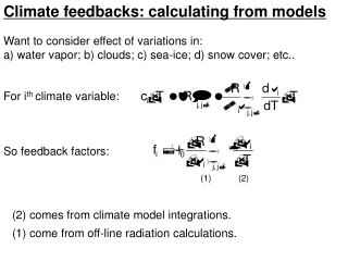
Climate feedbacks: calculating from models Want to consider effect of variations in: a) water vapor; b) clouds; c) sea-ice; d) snow cover; etc.. For ith climate variable: So feedback factors: (1) (2) (2) comes from climate model integrations. (1) come from off-line radiation calculations.
Climate feedbacks: estimating from models From suites of GCMS: Individual feedbacks uncorrelated among models, so can be simply combined: Soden & Held (2006): Colman (2003): • How does this uncertainty in physics translate to uncertainty in climate sensitivity?
Uncertainty: it all depends on where you are. Can show: T T for 2 x CO2 (oC) T f f • Uncertainty in climate sensitivity strongly dependent on the gain.
Climate sensitivity: the math Let pdf of uncertainty in feedbacks hf(f): Also have: So can write: Assume Gaussian h(f): Gives
Climate sensitivity: the picture for: • Skewed tail of high climate sensitivity is inevitable!
Climate sensitivity: an envelope of uncertainty 250,000+ integrations, 36,000,000+ yrs model time(!); Eqm. response of global, annual mean sfc. T to 2 x CO2. 6,000 model runs, perturbed physics Slab ocean, Q-flux 12 model params. varied • Two questions: • 1. What governs the shape of this distribution? • 2. How does uncertainty in physical processes translate into uncertainty in climate sensitivity?
Climate sensitivity: GCMs • GCMs produce climate sensitivity consistent with the • compounding effect of essentially-linear feedbacks.
Climate sensitivity: Observations and Models • works pretty well.
1. Climate sensitivity: can we do better? • How does uncertainty in climate sensitivity depend on f?
1. Climate sensitivity: can we do better? T science is here need to get here! • Not much change as a function of f
1. Climate sensitivity: can we do better? T science is here need to get here! • Not much change as a function of f
1. Climate sensitivity: can we do better? • Combination of mean feedback and uncertainty at which a given climate sensitivity can be rejected. • Need to get cross hairs below a given line to reject that T with 95% confidence
Climate Sensitivity: estimates over time Climate sensitivity Equilibrium change in global mean, annual mean temperature given CO2 2 x CO2 1. Arrhenius, 1896 2. Moller, 1963 3. Weatherald and Manabe, 1967 4. Manabe, 1971 5. Rasool and Schneider, 1971 6. Manabe and Weatherald, 1971 7. Sellers, 1974 8. Weare and Snell, 1974 9. NRC Charney report, 1979 10. IPCC1, 1990 11. Hoffert and Covey, 1992 12. IPCC2, 1996 13. Andronova & Schlesinger, 2001 14. IPCC3, 2001 15. Forest et al., 2002 16. Harvey & Kaufmann, 2002 17. Gregory et al., 2002 18. Murphy et al., 2004 19. Piani et al., 2005 20. Stainforth et al., 2005 21. Forest et al., 2006 22. Hegerl et al. 2006 23. IPCC4, 2007 24. Royer et al., 2007 • Why is uncertainty not diminishing with time?
4. Paleoclimate speculations? • What if feedback strengths change as a function of mean state? Eocene Proterozoic • Dramatic changes in physics are not necessary for dramatic • changes in climate sensitivity!
6. Climate at a point: the effect of random noise Can always expect random noise in the climate system: What is the effect of this noise on the behavior of the system? For time dep. eqn with random noise, dRf: Where (see review) rearranging Random forcing drives T' away from eqm. restoring ‘force’ - a relaxation back to equilibrium (T'=0)
6. Climate at a point: the effect of random noise Discretize eqn into time steps, t: Equation becomes where t is white noise current state random noise memory of last state - How does the system’s response to noise vary as a function of the memory, = (l,C, fi)?
6. Climate at a point: the effect of random noise t = 5 yrs t = 1 yr t = 25 yrs Time (yrs) The effect of varying t on the response of T’ to forcing by noise. note multi-decadal excursions here note century-scale excursions here The greater the memory, the longer the timescale of the variability
6. Climate at a point: the effect of random noise Climate is defined the statistics of weather. (i.e. the mean and standard deviation of atmospheric variables) Therefore a constant climate has a constant standard deviation (i.e., even in a constant climate there is variability) Crucial point: In paleoclimate, if the proxy variable (i.e., glacier, lake, tree, elephant, etc.) has long memory, say, t ~ 25 yrs, that proxy will have long timescale (i.e., centennial) variability even in a constant climate.
7. Climate at a point: power spectrum of response to noise amplitude time log(power) log(period=1/frequency) Quick intro to power spectra: they are an alternative way of describing a time series Time series Power spectrum Gives power (energy) at each sine wave frequency that makes up the time series (analogous to spectrum of light)
7. Climate at a point: power spectrum of response to noise t =1 yr log(power) t =5 yrs t =25 yrs log(period=1/frequency) Power spectra of response to noise as a function of t As there is more damping at high frequencies • The long t is, the ‘redder’ the power spectrum, • i.e., the greater the relative amount of long period variability.
7. Climate at a point: power spectrum of response to noise t =1 yr log(power) t =5 yrs t =25 yrs log(period=1/frequency) Eqn for this power spectra t • Can show 50% of power • in the spectrum occurs at • periods which are greater • than2 x . t t Crucial point. Long period variability is driven by short timescale physics.
7. Climate at a point: power spectrum of response to noise Why the factor of 2? i) Hand-wavy analogy with pendulum: Physical timescale Oscillation period ii) Real reason: Real time-behavior ~ Projected onto sines and cosines ~
8. Example: the Pacific Decadal Oscillation Dominant pattern of sea surface temperatures in North Pacific
8. Example: the Pacific Decadal Oscillation Power spectrum of PDO index Lots of variability at multi-decadal time scale But…. Best fit is a red noise process with a of 1.20.3 years i.e., indistinguishable from an annual timescale.
8. Example: the Pacific Decadal Oscillation PDO index Random noise & 1.2yr memory Random noise & 1.2yr memory [n.b. note the apparent long timescale variability even with short memory]
Examples from the modern climate The NAO The PNA The PDO 0 0.1 0.2 0.3 0.4 0.5 Frequency (/yr) Frequency (/yr)
Small print: In general, feedback strengths and sensitivity are functions of the mean state: For a black-body [Stefan-Boltzmann law] We linearized into A+BT: Our basic climate sensitivity: l0=1/B, is a sensitive function of T. Feedback analyses are completely linear, can be trouble when strongly nonlinear behavior is being studied. Feedback analyses rely on defining an appropriate reference state, against which to test models/observations. You have to be careful that the same reference state is being use when comparing feedbacks.
2. Nonlinearities in climate feedbacks. From basic analysis: But can take quadratic terms… Basic analysis: With quad. terms… • How might f’s change with mean state?
2. Nonlinearities in climate feedbacks • Stefan-Boltzmann relation: - longwave radiation ~ T4. - flw ~ 1/(4 T3) - negative feedback gets stronger with increasing T. b) Clausius-Clapeyron relation: - moisture content increases, so water vapor absorption bands fill up. - fwv~ 1/ esat d(esat(T))/dT - positive feedback becomes weaker with increasing T. Can show: f~0.02 for 4oC climate change Other nonlinear interactions: clouds = fn(sea-ice); snow albedo = fn(clouds); wat. vap. = fn(clouds), snow = fn(clouds); land sfc. albedo = fn(precip.); etc., etc. Easy to imagine a few nonlinear interactions giving f~0.1 ...
3. Are we stuck with a skewed distribution? • Could feedbacks vary enough with mean state • to remove skewness? Have that: To remove skewness would require: In other words would need f ~ -1.2 per 1oC (much stronger than is possible) • Skewed climate sensitivity distributions are intrinsic to system.
More curves changing playing with the uncertainty in climate feedbacks
More curves changing playing with the uncertainty in climate feedbacks