V. Latin squares designs (LS)
740 likes | 1.09k Vues
V. Latin squares designs (LS). V.A Design of Latin squares V.B Indicator-variable models and estimation for a Latin square V.C Hypothesis testing using the ANOVA method for a Latin square V.D Diagnostic checking V.E Treatment differences V.F Design of s ets of Latin square s

V. Latin squares designs (LS)
E N D
Presentation Transcript
V. Latin squares designs (LS) V.A Design of Latin squares V.B Indicator-variable models and estimation for a Latin square V.C Hypothesis testing using the ANOVA methodfor a Latin square V.D Diagnostic checking V.E Treatment differences V.F Design of sets of Latin squares V.G Hypothesis tests for sets of Latin squares Statistical Modelling Chapter V
V.A Design of Latin squares • Definition V.1: A Latin square design is one in which • each treatment occurs once and only once in each row and each column • so that the numbers of rows, columns and treatments are all equal. • Clearly, the total number of observations is n=t2. • Suppose in a field trial moisture is varying across the field and the stoniness down the field. • A Latin square can eliminate both sources of variability. Statistical Modelling Chapter V
Example V.1 Fertilizer experiment Statistical Modelling Chapter V
Notes • Even if one has not identified trends in two directions, a LS may be employed to guard against the problem of putting the blocks in the wrong direction. • LSs may also be used when there are two different kinds of blocking variables — for example animals and times. • General principle is to maximize row and column differences so as to minimize uncontrolled variation affecting treatment differences. • Problem is restriction that no. replicates = no. treats • Several fundamentally different LSs exist for a particular t • for t= 4 there are three different squares. • Latin squares for t= 3,4, ..., 9 given in Appendix 8A of Box, Hunter and Hunter. • To randomize these designs appropriately involves: • randomly select one of the Latin squares available for t; • randomly permute the rows and then the columns; • randomly assign letters to treatments. Statistical Modelling Chapter V
a) Obtaining a layout for a Latin Square in R • General instructions given in Appendix B, Randomized layouts and sample size computations in R. Example V.2 Pollution effects of petrol additives • 4 cars and 4 drivers in a study of effects of 4 petrol additives on pollution. • Desirable to isolate both car-to-car and driver-to-driver differences. • A 4 4 Latin square would enable this to be done. • Names for rows, columns and treats for this example are Cars, Drivers and Additives, respectively. • Also, t = 4 and a design obtained from BH2. Statistical Modelling Chapter V
Expressions to be used for example > t <- 4 > n <- t*t > LSPolut.unit <- list(Drivers=t, Cars=t) > Additives <- factor(c(1,2,3,4, 4,3,2,1, 2,4,1,3, 3,1,4,2), + labels=c("A","B","C","D")) > LSPolut.lay <- fac.layout(unrandomized=LSPolut.unit, + randomized=Additives,seed=941) > remove("Additives") > LSPolut.lay • Note: no nested.factors as Drivers and Cars are to be randomized independently • Hence they are not nested (are crossed) Statistical Modelling Chapter V
Randomized layout > LSPolut.lay Units Permutation Drivers Cars Additives 1 1 11 1 1 B 2 2 12 1 2 D 3 3 10 1 3 C 4 4 9 1 4 A 5 5 7 2 1 A 6 6 8 2 2 B 7 7 6 2 3 D 8 8 5 2 4 C 9 9 15 3 1 D 10 10 16 3 2 C 11 11 14 3 3 A 12 12 13 3 4 B 13 13 3 4 1 C 14 14 4 4 2 A 15 15 2 4 3 B 16 16 1 4 4 D Statistical Modelling Chapter V
V.B Indicator-variable models and estimation for a Latin square • Have to decide whether each of the factors Rows, Columns and Treatments are to be regarded as fixed or random. • As for the RCBD, it happens that the analysis of the Latin square is essentially unaffected by which model is used. • Generally, the Latin square involves t rows and columns so that there are n=t2 observations in all. Statistical Modelling Chapter V
a) Maximal model where Y is the t2-vector of random variables for the response variable observations, b is the t-vector of parameters specifying a different mean response for each row, XR is the t2t matrix indicating the row from which an observation came, d is the t-vector of parameters specifying a different mean response for each column, XC is the t2t matrix indicating the column from which an observation came, t is the t-vector of parameters specifying a different mean response for each treatment, XT is the t2tmatrix indicating the observations that received each of the treatments. • The maximal model when all are fixed, is • Our model also assumes Y ~ N(yR+C+T, V) Statistical Modelling Chapter V
Example V.3 A 33 Latin square • Suppose that a 33 Latin square with the following arrangement of treatments was being considered: • Then, for this example, • Note for general systematic layout XR=It1t and XC=1tIt but XTcannot be written as a direct product. Statistical Modelling Chapter V
are the t2-vectors of row, column, treatment and grand means, respectively. Estimators of expected values under max. model Also, note that • That is, MR, MC, MT and MG are the row, column, treatment and grand mean operators, respectively. • So once again the estimators are functions of means. • Further, if the data in the vector Y has been arranged in standard order for Rows then Columns, the operators are: In this case it is not possible to write MT as a direct product of I and J matrices as the treatments will not be in a systematicorder expressible in this form. Statistical Modelling Chapter V
Example V.3 A 33 Latin square (continued) Statistical Modelling Chapter V
b) Alternative expectation models • 8 possible different models for the expectation when Rows, Columns and Treatments are considered fixed: Statistical Modelling Chapter V
Marginality relations between the models • Estimators all are functions of the four mean vectors for this design Statistical Modelling Chapter V
V.C Hypothesis testing using the ANOVA method for a Latin square • An ANOVA will be used to choose between the 8 alternative expectation models for a Latin square. Statistical Modelling Chapter V
a) Analysis of an example • Example V.2 Pollution effects of petrol additives (continued) Statistical Modelling Chapter V
Hypothesis test for the example Step 1: Set up hypotheses a) H0: tA=tB=tC=tD (or XAt not required in model) H1: not all population Additives means are equal b) H0: bI=bII=bIII=bIV (or XDb not required in model) H1: not all population Drivers means are equal c) H0: d1=d2=d3=d4 (or XCd not required in model) H1: not all population Cars means are equal Set a= 0.05. Statistical Modelling Chapter V
Hypothesis test for the example (continued) Step 2: Calculate test statistics • Note Drivers#Cars refers to the "interaction between Drivers and Cars" • contrasts with Cars[Drivers] or Drivers[Cars]; • explained in chapter VII; • R does not distinguish as all are Drivers:Cars. Statistical Modelling Chapter V
Hypothesis test for the example (continued) Step 3: Decide between hypotheses Differences between drivers but not cars and differences between the additives. The model that best describes the data would appear to be yD+A = XDb + XAt, an additive model for Driver and Additive effects. Statistical Modelling Chapter V
b) Sums of squares for the analysis of variance • In this section we will use the generic names of Rows, Columns and Treatments for the factors in a Latin square. • The estimators of the SSqs for the Latin square ANOVA are the SSqs of the following vectors: • where • Ds are n-vectors of deviations from Y and • vectors with the e subscripts are n-vectors of effects. Statistical Modelling Chapter V
Ssq for the ANOVA (continued) • From section V.B, Models and estimation for a Latin square, • Can be shown that All the Ms and Qs are symmetric and idempotent. Statistical Modelling Chapter V
ANOVA table is constructed as follows: • See notes for example of computation of vectors and geometrical interpretation Statistical Modelling Chapter V
c) Expected mean squares • To justify our choice of test statistics, we want to work out the E[MSq]s in the ANOVA table under the 8 alternative expectation models. • However, to save space work out E[MSq]s under the maximal model and identify which terms in E[MSq]s go to zero under alternative models. Statistical Modelling Chapter V
E[MSq]s with fixed Rows and Columns effects • Given the expressions in the above table, the population means of the mean squares could be computed if knew the bis, djs, tks and s2. • Each of qR(y), qC(y) and qT(y) equal 0 when the terms XRb, XCd and XTt, respectively, removed from the model. • Hence a significant F value for a line indicates that the corresponding term should be included in the model. Statistical Modelling Chapter V
Alternative analysis • Both Rows and Columns are random • The model in this case would be that • It allows for equal covariance between units from the same row and also between units from the same column. Statistical Modelling Chapter V
Example V.3 A 33 Latin square (continued) Shows: Statistical Modelling Chapter V
Alternative variance models involve setting and/or and this will result in the one(s) set to zero being dropped from the expected mean square. E[MSq]s under alternative model • Alternative expectation model is yG=XGm and under this model qT(y) = 0. • This exactly parallelswhat happens when both are fixed. Statistical Modelling Chapter V
d) Summary of the hypothesis test • See notes e) Comparison with traditional Latin-square ANOVA table • Differences symbolic – see notes for details Statistical Modelling Chapter V
f) Computation of ANOVA and diagnostic checking in R • Diagnostic checking is the same as for the RCBD Example V.2 Pollution effects of petrol additives (continued) • First set up and attach data.frame and do initial boxplots. • Then, use the aov function, either with or without the Error as part of the model. • In this experiment uncontrolled variation made up of Drivers, Cars and Drivers:Cars. • R shorthand for this: Drivers*Cars that expands to Drivers + Cars + Drivers:Cars, the latter being equivalent to Drivers#Cars. • Outputs for analysis with Error & diagnostic checking are given below Statistical Modelling Chapter V
R output > load("LSPolut.dat.rda") > attach(LSPolut.dat) > boxplot(split(Reduct.NO, Drivers), xlab="Drivers", ylab="Reduction in NO") > boxplot(split(Reduct.NO, Cars), xlab="Cars", ylab="Reduction in NO") > boxplot(split(Reduct.NO, Additives), xlab="Additives", ylab="Reduction in NO") Statistical Modelling Chapter V
Boxplots for initial graphical exploration of the data Statistical Modelling Chapter V
R output (continued) < LSPolut.aov <- aov(Reduct.NO ~ Drivers + Cars + Additives + + Error(Drivers*Cars), LSPolut.dat) > summary(LSPolut.aov) Error: Drivers Df Sum Sq Mean Sq Drivers 3 216 72 Error: Cars Df Sum Sq Mean Sq Cars 3 24 8 Error: Drivers:Cars Df Sum Sq Mean Sq F value Pr(>F) Additives 3 40.000 13.333 5 0.0452 Residuals 6 16.000 2.667 > #Compute Drivers and Cars Fs and p-values > Drivers.F <- 72/2.667 > Drivers.p <- 1-pf(Drivers.F, 3, 6) > Cars.F <- 8/2.667 > Cars.p <- 1-pf(Cars.F, 3, 6) > data.frame(Drivers.F,Drivers.p,Cars.F,Cars.p) Drivers.F Drivers.p Cars.F Cars.p 1 26.99663 0.0006989578 2.999625 0.1169842 Statistical Modelling Chapter V
R output (continued) > # > # Diagnostic checking > # > res <- resid.errors(LSPolut.aov) > fit <- fitted.errors(LSPolut.aov) > data.frame(Drivers,Cars,Additives,Reduct.NO,res,fit) Drivers Cars Additives Reduct.NO res fit 1 1 1 B 20 1 19 2 1 2 D 20 1 19 3 1 3 C 17 -1 18 4 1 4 A 15 -1 16 5 2 1 A 20 -1 21 6 2 2 B 27 -1 28 7 2 3 D 23 1 22 8 2 4 C 26 1 25 9 3 1 D 20 -1 21 10 3 2 C 25 -1 26 11 3 3 A 21 1 20 12 3 4 B 26 1 25 13 4 1 C 16 1 15 14 4 2 A 16 1 15 15 4 3 B 15 -1 16 16 4 4 D 13 -1 14 Statistical Modelling Chapter V
R output (continued) > plot(fit, res, pch=16) > qqnorm(res, pch=16) > qqline(res) > tukey.1df(LSPolut.aov, LSPolut.dat, error.term = "Drivers:Cars") $Tukey.SS [1] 4.54224 $Tukey.F [1] 1.982167 $Tukey.p [1] 0.2181923 $Devn.SS [1] 11.45776 Statistical Modelling Chapter V
Hypothesis test for the example Step 1: Set up hypotheses (as before) a) H0: tA=tB=tC=tD (or XAt not required in model) H1: not all population Additives means are equal b) H0: bI=bII=bIII=bIV (or XDb not required in model) H1: not all population Drivers means are equal c) H0: d1=d2=d3=d4 (or XCd not required in model) H1: not all population Cars means are equal Set a= 0.05. Statistical Modelling Chapter V
Hypothesis test for the example (continued) Step 2: Calculate test statistics • Note inclusion of Nonadditivity Statistical Modelling Chapter V
Hypothesis test for the example (continued) Step 3: Decide between hypotheses As before, differences between drivers but not cars and differences between the additives. The model that best describes the data would appear to be yD+A = XDb + XAt, the additive model for Driver and Additive effects. The test for transformable nonadditivity is nonsignificant. Statistical Modelling Chapter V
Diagnostic checking • The residuals-versus-fitted-values plot indicates that the residuals are either -1 or 1 (must be artificial data). • Normal Probability Plot indicates that the data are not normal. • Clearly example can only be considered illustrative. Statistical Modelling Chapter V
IV.D Diagnostic checking • Again, we have assumed Y ~ N(y, s2I) where, for the maximal model, yR+C+T= E[Y] =XRb + XCd + XTt • For this model to be appropriate requires a similar set of behaviours as for the RCBD: • response is operating additively: a treatment has about the same additive effect on each unit; • variability of the units is the same for all row-column combinations; • each observation displays the covariance implied by the model (independence for Rows and Columns fixed; equal correlation within rows (columns) for Rows (Columns) random); and • that the response of the units is normally distributed. • As noted before, diagnostic checking same as for RCBD Statistical Modelling Chapter V
V.E Treatment differences • For the purposes of the scientist the effects of rows and columns are not of primary interest • Rather, focus on treatment differences. • Same as for CRD and RCBD. Example V.2 Pollution effects of petrol additives (continued) • As Additives significant, use Tukey's HSD procedure. Statistical Modelling Chapter V
Example V.2 Pollution effects of petrol additives (continued) > # multiple comparisons > # > model.tables(LSPolut.aov, type="means") Tables of means Grand mean 20 Drivers Drivers 1 2 3 4 23 24 15 18 Cars Cars 1 2 3 4 19 19 22 20 Additives Additives A B C D 18 22 21 19 > q <- qtukey(0.95, 4, 6) > q [1] 4.895599 • Comparing the differences in the additive means with Tukey’s HSD, it is concluded that only the difference between A and B are significant. Statistical Modelling Chapter V
Bar chart of Additives differences > # Plotting Treat means > LSPolut.tab <- model.tables(LSPolut.aov, type="means") > LSPolut.Adds.Mean <- data.frame(Adds.lev = levels(Additives), + Adds.Mean = as.vector(LSPolut.tab$tables$Additives)) > LSPolut.Adds.Mean <- LSPolut.Adds.Mean[order(LSPolut.Adds.Mean$Adds.Mean),] > LSPolut.Adds.Mean$Adds.lev <-factor(LSPolut.Adds.Mean$Adds.lev, + levels=LSPolut.Adds.Mean$Adds.lev) > barchart(Adds.Mean ~ Adds.lev, xlab="Additives", + ylim=c(0,25), ylab="NO Reduction", + main="Fitted values for Nitrous Oxide Reduction", + data=LSPolut.Adds.Mean) Note use of ylim to include 0 on y-axis Statistical Modelling Chapter V
V.F Design of sets of Latin squares • To overcome the small residual df problem several squares can be used. • In the case Example V.2, Pollution effects of petrol additives, Latin Square could be repeated using: • using the same drivers and cars in each replicate; • using the same drivers but new cars (or the same cars but new drivers); or • using new cars and drivers. • In general, one can have as many (r) squares as one likes. • However, will only present layouts for 2 squares. • General expressions for randomizing the various cases are given in Appendix B, Randomized layouts and sample size computations in R. Statistical Modelling Chapter V
Case 1 — same Drivers and Cars • This case involves a complete repetition of the experiment, say on consecutive mornings, with the same 4 Drivers and 4 Cars on the two occasions. • There is no re-randomization of the square for the second occasion — preserves crossed relationships between Occasions and other factors. • Layout (r=2) Statistical Modelling Chapter V
Case 2 — same cars different drivers • Experiment repeated on a different occasion with • same 4 cars on both occasions, • but with different drivers on second occasion. • As a result the rows of the square, but not the columns, are rerandomized on the second occasion. • Layout (r=2) • Note order in which additives are tested by second driver on occasion 1 is same as for fourth driver on occasion 2. • That is, the second row of the square on occasion 1 is the same as the fourth row on occasion 2. Statistical Modelling Chapter V
Case 3 — different drivers and cars • In this case, • not only are the drivers on different occasions unconnected, • but so are the cars as the cars used on the second occasion are completely different to those used on the first occasion. • As a result the rows and columns of the square are rerandomized on the second occasion. • Layout (r=2) Statistical Modelling Chapter V
V.G Hypothesis tests for sets of Latin squares • In previous section discussed the use of several squares to overcome the residual df problem. • e.g. 4 4 Latin square has 6 (< 10) Residual df • Gave 3 cases for Example V.2, Pollution effects of petrol additives: • using the same drivers and cars in each replicate; • using the same drivers but new cars (or the same cars but new drivers); or • using new cars and drivers. • Shall determine ANOVA for each of these cases. • In determining the E[MSq]s will be assumed that • unrandomized factors are to be classified as random factors • randomized factors as fixed factors. • While layouts were for 2 squares will give DF for the general case of r squares. Statistical Modelling Chapter V
a) Case 1 — same Drivers and Cars • no re-randomization of the square for the second occasion • Layout (r=2) Statistical Modelling Chapter V
A. Description of pertinent features of the study • Observational unit • a car with a driver on an occasion • Response variable • Reduction • Unrandomized factors • Occasions, Drivers, Cars • Randomized factors • Additives • Type of study • Sets of Latin Squares Statistical Modelling Chapter V
B. The experimental structure • For this structure to be appropriate requires that the same square without re-randomization be used for each occasions; otherwise, some factors would be nested (as would be randomizing within Occasions). C. Sources derived from the structure formulae Occasions*Drivers*Cars = (Occasions + Drivers + Occasions#Drivers)*Cars = Occasions + Drivers + Occasions#Drivers + Cars + Occasions#Cars + Drivers#Cars + Occasions#Drivers#Cars Additives = Additives Statistical Modelling Chapter V