CSC 213
CSC 213. Lecture 24: Minimum Spanning Trees. Announcements. Final exam is: Thurs. 5/11 from 8:30-10:30AM in Old Main 205. Spanning subgraph Subgraph including every vertex Spanning tree Spanning subgraph that is also a tree Minimum spanning tree

CSC 213
E N D
Presentation Transcript
CSC 213 Lecture 24:Minimum Spanning Trees
Announcements • Final exam is: Thurs. 5/11 from 8:30-10:30AM in Old Main 205
Spanning subgraph Subgraph including every vertex Spanning tree Spanning subgraph that is also a tree Minimum spanning tree Spanning tree with minimum total edge weight Minimum Spanning Tree (MST) ORD 10 1 PIT DEN 6 7 9 3 DCA STL 4 5 8 2 DFW ATL
8 f 4 C 9 6 2 3 e 7 8 7 8 f 4 C 9 6 2 3 e 7 8 7 Cycle Property Cycle Property: • MSTs do not contain cycles • So weight of each edge in MST is lower than weight of edge which completes cycle Proof: • e is edge in G¬ in MST • C is cycle formed when adding e to MST • For every edge f in C,weight(f) weight(e) • If weight(f)> weight(e),then exists a smaller spanning tree with e instead of f Replacing f with e yieldsa better spanning tree
Partition Property U V 7 f 4 Partition Property: • Given partitions of vertices, minimum weight edge is in a MST connecting partitions Proof: • e is edge with smallest weight connecting partitions, but not in MST • f connects partitions in MST • If MST does not contain e, consider cycle formed by including e with MST • By cycle property,weight(f)≤ weight(e) • But since e has smallest weight,weight(f) =weight(e) • Create another MST by replacing f with e 9 5 2 8 3 8 e 7 Replacing f with e yieldsanother MST U V 7 f 4 9 5 2 8 3 8 e 7
Kruskal’s Algorithm • Add edges to MST greedily • Priority queue contains edges outside the cloud • Element: edge • Key: edge’s weight • Only want edges that will not make a cycle • Unfortunately, detecting cycles can be hard…
Data Structs for Kruskal Algorithm • Algorithm maintains forest of trees • Edge accepted when connecting trees • Use partition (i.e., collection of disjoint sets): • find(u): return set containing u • union(u,v): replace sets with u & v with their union
Partition Representation • Each set is Sequence • Each element refers to its set • makeSet(u) takes O(1) time • find(u) takes O(1) time • union(u,v) moves elements of smaller set to Sequence of larger set and updates references • By having union move smaller set into large set, elements are processed only when set size doubles • n calls to union() takes O(log n) time
Kruskal’s Algorithm AlgorithmKruskalMST(Graph G) Q newPriorityQueue() T newGraph() P newPartition() for each vertex v in G P.makeSet(v) T.insertVertex(v) for each edge e in G Q.insert(e.getWeight(), e); whileT.edges().getSize() < n-1 Edge e = Q.removeMin() Assign u, v to G.endpoints(e) ifP.find(u)P.find(v)then T.insertEdge(e) P.union(P.find(u),P.find(v)) returnT
Kruskal Example 2704 BOS 867 849 PVD ORD 187 740 144 JFK 1846 621 1258 184 802 SFO BWI 1391 1464 337 1090 DFW 946 LAX 1235 1121 MIA 2342
2704 BOS 867 849 PVD ORD 187 JFK 1258 SFO BWI DFW LAX MIA Example 740 144 1846 621 184 802 1391 1464 337 1090 946 1235 1121 2342
Prim-Jarnik’s Algorithm • Similar to Dijkstra’s algorithm • Pick arbitrary vertex s and grow MST as cloud of vertices • Label each vertex v with d(v) --- smallest weight of edge connecting v to vertex in cloud • At each step: • Add vertex u with smallest distance to cloud • Update labels of vertices adjacent to u
Prim-Jarnik’s Algorithm (cont.) • Priority queue stores vertices outside of cloud • Key: distance • Element: vertex • Locator-based methods • insert(k,e) – returns locator • replaceKey(l,k) – changes item’s key • Store three labels with each vertex • Distance from cloud • Edge connecting vertex to cloud (MST edge) • Locator in priority queue
Prim-Jarnik’s Algorithm (cont.) AlgorithmPrimJarnikMST(Graph G) Q newPriorityQueue() s G.vertices().elemAtRank(0) for each vertex v in G ifv= s v.setDistance(0) else v.setDistance() v.setParent(null) l Q.insert(getDistance(v),v) setLocator(v,l) while !Q.isEmpty() u Q.removeMin() for each edge e in G.incidentEdges(u) z G.opposite(u,e) r e.getWeight() ifr< z.getDistance() z.setDistance(r) z.setParent(e)Q.replaceKey(z.getLocator(),r)
Example 7 7 D 7 D 2 2 B B 4 4 9 9 8 5 5 5 F F 2 2 C C 8 8 3 3 8 8 E E A A 7 7 7 7 0 0 7 7 7 D 2 7 D 2 B 4 B 4 9 5 4 9 5 5 F 2 5 F 2 C 8 C 8 3 3 8 8 E E A 7 7 A 7 0 7 0
Example (contd.) 7 7 D 2 B 4 4 9 5 5 F 2 C 8 3 8 E A 3 7 7 0 7 D 2 B 4 4 9 5 5 F 2 C 8 3 8 E A 3 7 0
Prim-Jarnik’s Analysis • Operations • incidentEdges called once per vertex • Set/Get each vertex’s labels O(deg(v)) times • Priority queue operations • Each vertex inserted once and removed once • Each insertion/removal takes O(log n) • Vertex w’skey modified O(deg(w)) times • Each key change takes O(log n) time • Algorithm takes O((n + m) log n) time using adjacency list structure