Measuring Atmospheric Parameters with SuperBeams

1. Measuring Atmospheric Parameters with SuperBeams Enrique Fernández Martínez Departamento de Física Teórica and IFT Universidad Autónoma de Madrid

2. Outline • Introduction • Oscillation parameters • Experiments description • Subleading effects in nm disappearance • Dm2atm and the sign degeneracy • q23 and the octant degeneracy • The effects of q13 and d • T2K-1 bounds revised • Conclusions

3. The oscillation parameters • What we already know • Solar sector • Atm sector • What we still don’t know • sin2q13< 0.40 • dcp • Mass hierarchy • Octant ofq23 q12 = 28º–38º q23 = 35º–55º M. C. González García hep-ph/0410030

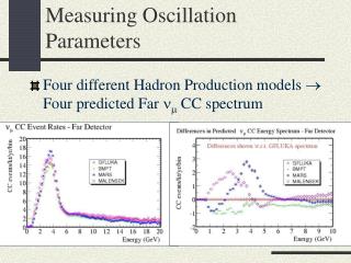
4. flux from p+ decay flux from p- decay Fluxes T2K-1 SPL OA2º L=295Km L=130Km flux from p+ decay at Old SPL fluxes courtesy of Gilardoni New fluxes Campagne et al. hep-ex/0411062 T2K fluxes courtesy of J.J. Gómez Cadenas

5. 5yr exposure with a 22.5Kt water cerenkov detector for T2K-1 2yr + 8yr exposure with a 440Kt water cerenkov detector for the SPL Event Rates 4 energy bins of 200MeV Between 0.4 – 1.2GeV L=130Km L=295Km Statisticsdominated Systematics dominated

6. The importance of energy resolution T2K-1 SPL q13 = 0º d = 0º 90% CL contours 5% systematic error and backgrounds taken into account

7. = E 0 . 27 GeV n The importance of energy resolution T2K-1 SPL q13 = 0º d = 0º

8. = E 0 . 27 GeV n = E 0 . 25 GeV n The importance of energy resolution T2K-1 SPL q13 = 0º d = 0º E1 = 0.4 - 0.6GeV

9. = E 0 . 27 GeV n = E 0 . 25 GeV n The importance of energy resolution T2K-1 SPL q13 = 0º d = 0º E1 = 0.4 - 0.6GeV E2 = 0.6 - 0.8GeV

10. = E 0 . 27 GeV n = E 0 . 25 GeV n The importance of energy resolution T2K-1 SPL q13 = 0º d = 0º E1 = 0.4 - 0.6GeV E2 = 0.6 - 0.8GeV E3 = 0.8 - 1.0GeV

11. = E 0 . 27 GeV n = E 0 . 25 GeV n The importance of energy resolution T2K-1 SPL q13 = 0º d = 0º E1 = 0.4 - 0.6GeV E2 = 0.6 - 0.8GeV E3 = 0.8 - 1.0GeV E4 = 1.0 - 1.2GeV

12. = E 0 . 27 GeV n = E 0 . 25 GeV n The importance of energy resolution T2K-1 SPL q13 = 0º d = 0º E1 = 0.4 - 0.6GeV E2 = 0.6 - 0.8GeV E3 = 0.8 - 1.0GeV E4 = 1.0 - 1.2GeV

13. D æ ö L ( ) - - 2 2 2 2 ç ÷ atm q q q 1 sin 2 s sin 2 cos 2 sin2 23 23 13 23 2 è ø D æ ö L ~ ( ) [ ] - + D 2 2 2 ç ÷ sol s sin 2 q J s cos d sin L 12 23 23 atm 2 è ø 2 D æ ö L ( ) ] [ - + D 4 2 2 2 ç ÷ sol q q c sin 2 s sin 2 cos L 23 12 12 23 atm 2 è ø D 2 m D = ~ 12 = q q q q J cos sin 2 sin 2 sin 2 sol 2 E 13 13 12 23 D D æ ö 2 L m @ D = ç ÷ sol 0 . 05 23 atm 2 2 E è ø The nm disappearance channel Where sin 2q13 < 0.4 E. K. Akhmedov et al.hep-ph/0402175 A. Donini et al.hep-ph/0411402

14. D æ ö L ( ) - 2 ç ÷ atm q 1 sin 2 sin2 23 2 è ø D æ ö L + O ç ÷ sol 2 è ø 2 D æ ö L + O ç ÷ sol 2 è ø The sign degeneracy Input: q13 = 0º d = 0º

15. D æ ö L ( ) - 2 ç ÷ atm q 1 sin 2 sin2 23 2 è ø D æ ö L ( ) [ ] - D 2 2 ç ÷ sol s sin 2 q sin L 12 23 atm 2 è ø 2 D æ ö L + O ç ÷ sol 2 è ø The sign degeneracy Input: q13 = 0º d = 0º

16. D æ ö L ( ) - 2 ç ÷ atm q 1 sin 2 sin2 23 2 è ø D æ ö L ( ) [ ] - D 2 2 ç ÷ sol s sin 2 q sin L 12 23 atm 2 è ø 2 D æ ö L + O ç ÷ sol 2 è ø The sign degeneracy Input: q13 = 0º d = 0º Fit assuming inverted hierarchy

17. D æ ö L ( ) - 2 ç ÷ atm q 1 sin 2 sin2 23 2 è ø D æ ö L ( ) [ ] - D 2 2 ç ÷ sol s sin 2 q sin L 12 23 atm 2 è ø 2 D æ ö L + O ç ÷ sol 2 è ø The octant degeneracy Input: q13 = 0º d = 0º

18. D æ ö L ( ) - 2 ç ÷ atm q 1 sin 2 sin2 23 2 è ø D æ ö L ( ) [ ] - D 2 2 ç ÷ sol s sin 2 q sin L 12 23 atm 2 è ø 2 D æ ö L + O ç ÷ sol 2 è ø The octant degeneracy Input: q13 = 0º d = 0º

19. D æ ö L ( ) - 2 ç ÷ atm q 1 sin 2 sin2 23 2 è ø D æ ö L ( ) [ ] - D 2 2 ç ÷ sol s sin 2 q sin L 12 23 atm 2 è ø 2 D æ ö L + O ç ÷ sol 2 è ø The effect of q13 Input: q13 = 0º d = 0º

20. D æ ö L ( ) - - 2 2 2 2 ç ÷ atm q q q 1 sin 2 s sin 2 cos 2 sin2 23 23 13 23 2 è ø D æ ö L ~ ( ) [ ] - + D 2 2 2 ç ÷ sol s sin 2 q J s cos d sin L 12 23 23 atm 2 è ø 2 D æ ö L + O ç ÷ sol 2 è ø The effect of q13 Input: q13 = 0º d = 0º Assuming q13 = 0º

21. D æ ö L ( ) - - 2 2 2 2 ç ÷ atm q q q 1 sin 2 s sin 2 cos 2 sin2 23 23 13 23 2 è ø D æ ö L ~ ( ) [ ] - + D 2 2 2 ç ÷ sol s sin 2 q J s cos d sin L 12 23 23 atm 2 è ø 2 D æ ö L + O ç ÷ sol 2 è ø The effect of q13 Input: q13 = 0º d = 0º Assuming q13 = 0º, 2º

22. D æ ö L ( ) - - 2 2 2 2 ç ÷ atm q q q 1 sin 2 s sin 2 cos 2 sin2 23 23 13 23 2 è ø D æ ö L ~ ( ) [ ] - + D 2 2 2 ç ÷ sol s sin 2 q J s cos d sin L 12 23 23 atm 2 è ø 2 D æ ö L + O ç ÷ sol 2 è ø The effect of q13 Input: q13 = 0º d = 0º Assuming q13 = 0º, 2º, 4º

23. D æ ö L ( ) - - 2 2 2 2 ç ÷ atm q q q 1 sin 2 s sin 2 cos 2 sin2 23 23 13 23 2 è ø D æ ö L ~ ( ) [ ] - + D 2 2 2 ç ÷ sol s sin 2 q J s cos d sin L 12 23 23 atm 2 è ø 2 D æ ö L + O ç ÷ sol 2 è ø The effect of q13 Input: q13 = 0º d = 0º Assuming q13 = 0º, 2º, 4º, 6º

24. D æ ö L ( ) - - 2 2 2 2 ç ÷ atm q q q 1 sin 2 s sin 2 cos 2 sin2 23 23 13 23 2 è ø D æ ö L ~ ( ) [ ] - + D 2 2 2 ç ÷ sol s sin 2 q J s cos d sin L 12 23 23 atm 2 è ø 2 D æ ö L + O ç ÷ sol 2 è ø The effect of q13 Input: q13 = 0º d = 0º Assuming q13 = 0º, 2º, 4º, 6º, 8º

25. D æ ö L ( ) - - 2 2 2 2 ç ÷ atm q q q 1 sin 2 s sin 2 cos 2 sin2 23 23 13 23 2 è ø D æ ö L ~ ( ) [ ] - + D 2 2 2 ç ÷ sol s sin 2 q J s cos d sin L 12 23 23 atm 2 è ø 2 D æ ö L + O ç ÷ sol 2 è ø The effect of q13 Input: q13 = 0º d = 0º Assuming q13 = 0º, 2º, 4º, 6º, 8º, 10º

26. D æ ö L ( ) - - 2 2 2 2 ç ÷ atm q q q 1 sin 2 s sin 2 cos 2 sin2 23 23 13 23 2 è ø D æ ö L ~ ( ) [ ] - + D 2 2 2 ç ÷ sol s sin 2 q J s cos d sin L 12 23 23 atm 2 è ø 2 D æ ö L + O ç ÷ sol 2 è ø The effect of d Input: q13 = 8º d = 0º Assuming d = 0º

27. D æ ö L ( ) - - 2 2 2 2 ç ÷ atm q q q 1 sin 2 s sin 2 cos 2 sin2 23 23 13 23 2 è ø D æ ö L ~ ( ) [ ] - + D 2 2 2 ç ÷ sol s sin 2 q J s cos d sin L 12 23 23 atm 2 è ø 2 D æ ö L + O ç ÷ sol 2 è ø The effect ofd Input: q13 = 8º d = 0º Assuming d = 0º, 90º

28. D æ ö L ( ) - - 2 2 2 2 ç ÷ atm q q q 1 sin 2 s sin 2 cos 2 sin2 23 23 13 23 2 è ø D æ ö L ~ ( ) [ ] - + D 2 2 2 ç ÷ sol s sin 2 q J s cos d sin L 12 23 23 atm 2 è ø 2 D æ ö L + O ç ÷ sol 2 è ø The effect of d Input: q13 = 8º d = 0º Assuming d = 0º, 90º, 180º

29. T2K-1 errors revised Input: q13 = 0º q23 = 45º d = 0º 90% CL Present: Dm2 = (1.7 – 3.5)·10-3 eV2 sin22q> 0.9 tan2q= 0.53 – 2.04 Dm2 = (2.50 ± 0.06)·10-3 eV2 sin22q> 0.98 Y. Itow et al.hep-ex/0106019 Dm2 = (2.43 – 2.60)·10-3 eV2 sin22q> 0.97 tan2q= 0.73 – 1.39 Dm2 = (2.45 – 2.56)·10-3 eV2 sin22q> 0.98 tan2q= 0.76 – 1.31 Dm2 = (-2.63 – -2.49)·10-3 eV2

30. T2K-1 errors revised Input: q13 = 0º q23 = 40º d = 0º 90% CL Present: Dm2 = (1.7 – 3.5)·10-3 eV2 sin22q> 0.9 tan2q= 0.53 – 2.04 Dm2 = (2.42 – 2.61)·10-3 eV2 sin22q= 0.94 – 0.99 tan2q= 0.62 – 0.85, 1.21 – 1.66 Dm2 = (2.44 – 2.58)·10-3 eV2 sin22q= 0.95 – 0.99 tan2q= 0.63 – 0.81,1.24 – 1.58 Dm2 = (-2.64 – -2.47)·10-3 eV2

31. Conclusions • The measurement of q13and dwill rely heavily on an improvement of the measure of q23 and Dm223 • Precision measurements of q23 and Dm223 need energy resolution and events above and below the oscillation peak • The errors on the q23and Dm223 are somewhat larger due to the dependence of the disappearance signal on q13, dand the mass hierarchy • This dependence can be exploited combined with the appearance channel to solve degeneracies

32. T2K-2 T2K-1 T2K-2 5% systematic error

33. T2K-2 T2K-1 T2K-2 2% systematic error

34. No background and no systematic Systematic 5% With Background Systematic 0% No Background Errors dominated by statistics

35. 10% systematic Systematic 5% Systematic 10% Errors dominated by statistics

36. Energy Resolution Figure taken from Y. Itow et al.hep-ex/0106019 Red histogram for true QE events

37. Double energy resolution 8 bins of 100MeV 4 bins of 200MeV

38. Double energy resolution 8 bins of 100MeV 4 bins of 200MeV