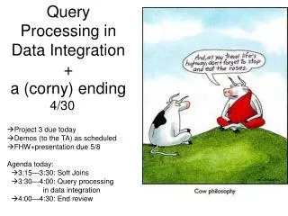
Query Processing in Data Integration (Gathering and Using Source Statistics)
Query Processing in Data Integration (Gathering and Using Source Statistics). Query Optimization Challenges. -- Deciding what to optimize --Getting the statistics on sources --Doing the optimization. Information Integration. Text/Data Integration. Service integration. Data Integration.

Query Processing in Data Integration (Gathering and Using Source Statistics)
E N D
Presentation Transcript
Query Processing in Data Integration(Gathering and Using Source Statistics)
Query Optimization Challenges -- Deciding what to optimize --Getting the statistics on sources --Doing the optimization
Information Integration Text/Data Integration Service integration Data Integration Collection Selection Data aggregation (vertical integration) Data Linking (horizontal integration)
Fully automated II (blue sky for now) Get a query from the user on the mediator schema Go “discover” relevant data sources Figure out their “schemas” Map the schemas on to the mediator schema Reformulate the user query into data source queries Optimize and execute the queries Return the answers Fully hand-coded II Decide on the only query you want to support Write a (java)script that supports the query by accessing specific (pre-determined) sources, piping results (through known APIs) to specific other sources Examples include Google Map Mashups Extremes of automation in Information Integration (most interesting action is “in between”) E.g. We may start with known sources and their known schemas, do hand-mapping and support automated reformulation and optimization
What to Optimize • Traditional DB optimizers compare candidate plans purely in terms of the time they take to produce all answers to a query. • In Integration scenarios, the optimization is “multi-objective” • Total time of execution • Cost to first few tuples • Often, the users are happier with plans that give first tuples faster • Coverage of the plan • Full coverage is no longer an iron-clad requirement • Too many relevant sources, Uncontrolled overlap between the sources • Can’t call them all! • (Robustness, • Access premiums…)
Roadmap • We will first focus on optimization issues in vertical integration (“data aggregation” ) scenarios • Learning source statistics • Using them to do source selection • Then move to optimization issues in horizontal integration (“data linking”) scenarios. • Join optimization issues in data integration scenarios
Query Processing Issues in Data Aggregation • Recall that in DA, all sources are exporting fragments of the same relation R • E.g. Employment opps; bibliography records; item/price records etc • The fragment of R exported by a source may have fewer columns and/or fewer rows • The main issue in DA is “Source Selection” • Given a query q, which source(s) should be selected and in what order • Objective: Call the least number of sources that will give most number of high-quality tuples in the least amount of time • Decision version: Call k sources that …. • Quality of tuples– may be domain specific (e.g. give lowest price records) or domain independent (e.g. give tuples with fewest null values)
Issues affecting Source Selection in DA • Source Overlap • In most cases you want to avoid calling overlapping sources • …but in some cases you want to call overlapping sources • E.g. to get as much information about a tuple as possible; to get the lowest priced tuple etc. • Source latency • You want to call sources that are likely to respond fast • Source quality • You want to call sources that have high quality data • Domain independent: E.g. High density (fewer null values) • Domain specific E.g. sources having lower cost books • Source “consistency”? • Exports data that is error free
Learning Source Statistics • Coverage, overlap, latency, density and quality statistics about sources are not likely to be exported by sources! • Need to learn them • Most of the statistics are source and query specific • Coverage and Overlap of a source may depend on the query • Latency may depend on the query • Density may depend on the query • Statistics can be learned in a qualitative or quantitative way • LCW vs. coverage/overlap statistics • Feasible access patterns vs. binding pattern specific latency statistics • Quantitative is more general and amenable to learning • Too costly to learn statistics w.r.t. each specific query • Challenge: Find right type of query classes with respect to which statistics are learned • Query class definition may depend on the type of statistics • Since sources, user population and network are all changing, statistics need to be maintained (through incremental changes)
Managing Source Overlap • Often, sources on the Internet have overlapping contents • The overlap is notcentrally managed (unlike DDBMS—data replication etc.) • Reasoning about overlap is important for plan optimality • We cannot possibly call all potentially relevant sources! • Qns: How do we characterize, get and exploit source overlap? • Qualitative approaches (LCW statements) • Quantitative approaches (Coverage/Overlap statistics)
Local Completeness Information • If sources are incomplete, we need to look at each one of them. • Often, sources are locally complete. • Movie(title, director, year) complete for years after 1960, or for American directors. • Question: given a set of local completeness statements, is a query Q’ a complete answer to Q? Problems: 1. Sources may not be interested in giving these! Need to learn hard to learn! 2. Even if sources are willing to give, there may not be any “big enough” LCWs Saying “I definitely have the car with vehicle ID XXX is useless Advertised description True source contents Guarantees (LCW; Inter-source comparisons)
Quantitative ways of modeling inter-source overlap • Coverage & Overlap statistics [Koller et. al., 97] • S1 has 80% of the movies made after 1960; while S2 has 60% of the movies • S1 has 98% of the movies stored in S2 • Computing cardinalities of unions given intersections • Who gives these statistics? • -Third party • -Probing
BibFinder: A popular CS bibliographic mediator Integrating 8 online sources: DBLP, ACM DL, ACM Guide, IEEE Xplore, ScienceDirect, Network Bibliography, CSB, CiteSeer More than 58000 real user queries collected Mediated schema relation in BibFinder: paper(title, author, conference/journal, year) Primary key: title+author+year Focus on Selection queries Q(title, author, year) :- paper(title, author, conference/journal, year), conference=SIGMOD Case Study: BibFinder
Selecting top-K sources for a given query • Given a query Q, and sources S1….Sn, we need the coverage and overlap statistics of sources Si w.r.t. Q • P(S|Q) is the coverage (Probability that a random tuple belonging to Q is exported by source S) • P({S1..Sj}|Q) is the overlap between S1..Sj w.r.t. query Q (Probability that a random tuple belonging to Q is exported by all the sources S1..Sj). • If we have the coverage and overlap statistics, then it is possible to pick the top-K sources that will give maximal number of tuples for Q.
Computing Effective Coverage provided by a set of sources Suppose we are calling 3 sources S1, S2, S3 to answer a query Q. The effective coverage we get is P(S1US2US3|Q). In order to compute this union, we need the intersection (overlap) statistics (in addition to the coverage statistics) Given the above, we can pick the optimal 3-sources for answering Q by considering all 3-sized subsets of source set S1….Sn, and picking the set with highest coverage
Selecting top-K sources: the greedy way Selecting optimal K sources is hard in general. One way to reduce cost is to select sources greedily, one after other. For example, to select 3 sources, we select first source Si as the source with highest P(Si|Q) value. To pick the jth source, we will compute the residual coverage of each of the remaining sources, given the 1,2…j-1 sources we have already picked The residual coverage computation requires overlap statistics). For example picking a third source in the context of sources S1 and S2 will require us to calculate:
Challenges in gathering overlap statistics • Sources are incomplete and partially overlapping • Calling every possible source isinefficient and impolite • Need coverage and overlap statistics to figure out what sources are most relevant for every possible query! • We introduce a frequency-based approach for mining these statistics
Outline • Motivation • BibFinder/StatMiner Architecture • StatMiner Approach • Automatically learning AV Hierarchies • Discovering frequent query classes • Learning coverage and overlap Statistics • Using Coverage and Overlap Statistics • StatMiner evaluation with BibFinder • Related Work • Conclusion
Challenges of gathering coverage and overlap statistics • It’s impractical to assume that the sources will export such statistics, because the sources are autonomous. • It’s impractical to learn and store all the statistics for every query. • Necessitate different statistics, is the number possible queries, is the number of sources • Impractical to assume knowledge of entire query population a priori Motivation • We introduce StatMiner • A threshold based hierarchical mining approach • Store statistics w.r.t. query classes • Keep more accurate statistics for more frequently asked queries • Handling the efficiency and accuracy tradeoffs by adjusting the thresholds
Query List • Each query q corresponds to a • Vector of coverage/overlap • Statistics. If there are 3 sources • S1, s2, s3, we have: • [P(S1|q),P(S2|q), P(S3|q) • P(S1&S2|q), P(S2&S3|q) P(S1&S3|q) • P(S1&S2&S3|q) ] • A sparse vector with exponential • dimensions • By keeping thresholds on min • overlap, we can avoid remembering • small values • The larger the thresholds, the sparser • the vectors
Issues in Storing & Using Statistics • Storing statistics for each query is disadvantageous • Too many queries • Stored statistics can only be useful if the same query comes up again • Idea1: Focus on only frequently asked queries • Idea 2: Store statistics w.r.t. query classes • Generate query classes by clustering.. • When a new query comes, we can map it to some existing query classes • But Clustering directly on queries won’t work • Because we won’t know how to map a new query into existing query classes • Idea: First do “subspace” clustering—cluster attribute values • A query class is then defined as a cross product of attribute value clusters
StatMiner A query is a vector of overlap statistics
Outline • Motivation • BibFinder/StatMiner Architecture • StatMiner Approach • Automatically learning AV Hierarchies • Discovering frequent query classes • Learning coverage and overlap Statistics • Using Coverage and Overlap Statistics • StatMiner evaluation with BibFinder • Related Work • Conclusion
BibFinder/StatMiner Evaluation • Experimental setup with BibFinder: • Mediator relation: Paper(title,author,conference/journal,year) • 25000 real user queries are used. Among them 4500 queries are randomly chosen as test queries. • AV Hierarchies for all of the four attributes are learned automatically. • 8000 distinct values in author, 1200 frequent asked keywords itemsets in title, 600 distinct values in conference/journal, and 95 distinct values in year.
Space Consumption for Different minfreq and minoverlap • We use a threshold on the support of a class, called minfreq, to identify frequent classes • We use a minimum support threshold minoverlap to prune overlap statistics for uncorrelated source sets. • As we increase any of the these two thresholds, the memory consumption drops, especially in the beginning.
Accuracy of the Learned Statistics • Absolute Error • No dramatic increases • Keeping very detailed overlap statistics would not necessarily increase the accuracy while requiring much more space. For example: minfreq=0.13 and minoverlap=0.1 versus minfreq=0.33 and minoverlap=0
Plan Precision • Here we observe the average precision of the top-2 source plans • The plans using our learned statistics have high precision compared to random select, and it decreases very slowly as we change the minfreq and minoverlap threshold.
Plan Precision on Controlled Sources We observer the plan precision of top-5 source plans (totally 25 simulated sources). Using greedy select do produce better plans. See Section 3.8 and Section 3.9 for detailed information
Number of Distinct Results • Here we observe the average number of distinct results of top-2 source plans. • Our methods gets on average 50 distinct answers, while random search gets only about 30 answers.
Latency statistics(Or what good is coverage without good response time?) • Sources vary significantly in terms of their response times • The response time depends both on the source itself, as well as the query that is asked of it • Specifically, what fields are bound in the selection query can make a difference • ..So, learn statistics w.r.t. binding patterns
Query Binding Patterns • A binding pattern refers to which arguments of a relational query are “bound” • Given a relation S(X,Y,Z) • A query S(“Rao”, Y, “Tom”) has binding pattern bfb • A query S(X,Y, “TOM”) has binding pattern ffb • Binding patterns can be generalized to take “types” of bindings • E.g. S(X,Y,1) may be ffn (n being numeric binding) and • S(X,Y, “TOM”) may be ffs (s being string binding) • Sources tend to have different latencies based on the binding pattern • In extreme cases, certain binding patterns may have infinite latency (i.e., you are not allowed to ask that query) • Called “infeasible” binding patterns
(Digression) • LCWs are the “qualitative” versions of quantitative coverage/overlap statistics • Feasible binding patterns are “qualitative” versions of quantitative latency statistics
Combining coverage and response time • Qn: How do we define an optimal plan in the context of both coverage/overlap and response time requirements? • An instance of “multi-objective” optimization • General solution involves presenting a set of “pareto-optimal” solutions to the user and let her decide • Pareto-optimal set is a set of solutions where no solution is dominated by another one in all optimization dimensions (i.e., both better coverage and lower response time) • Another idea is to combine both objectives into a single weighted objective