EVOLUTION AND INTERNAL STRUCTURE OF RED GIANTS
650 likes | 802 Vues
EVOLUTION AND INTERNAL STRUCTURE OF RED GIANTS. Maurizio Salaris Astrophysics Research Institute Liverpool John Moores University. What stars am I going to talk about?. Kallinger et al. (2010). Adapted from Gallart (1999). From McConnachie et al. (2006). RGB stars as metallicity indicators.

EVOLUTION AND INTERNAL STRUCTURE OF RED GIANTS
E N D
Presentation Transcript
EVOLUTION AND INTERNAL STRUCTURE OF RED GIANTS Maurizio Salaris Astrophysics Research Institute Liverpool John Moores University
What stars am I going to talk about? Kallinger et al. (2010) Adapted from Gallart (1999)
From McConnachie et al. (2006) RGB stars as metallicity indicators ↓ RC stars as SFH diagnostics ←
14Gyr 10 [Fe/H]= −0.7 −0.35 +0.06 +0.40 Number of RGB stars above the HB level reduced by a factor 2 8 6 3 Blue circles Teff + 100 K (only RGB)
OUTLINE • The three classes of red giant stars • Behaviour in the CMD (or HRD) • Internal structure • Some long-standing uncertainties • Examples of applications to more general astrophysical problems
Representative evolutionary tracks Solar initial chemical composition 1.0 Mo 2.4 Mo EAGB RC RGB
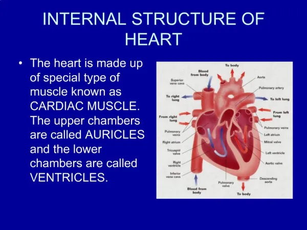
RGB stars • Objects with (initial) mass lower than ~2.0Mo • Electron degenerate (nearly) isothermal He-core surrounded by a thin (~0.001-0.0001 Mo thickness) H-burning shell that is, in turn, surrounded by an extended convective envelope • Evolution towards increasing luminosity and moderately decreasing Teff due to the steady increase of the He-core mass • Efficient mass loss from the convective envelope • He-flash terminates RGB evolution when McHe~0.47 - 0.50Mo
RGB in the CMD (or HRD) age metallicity initial helium Lbol of the TRGB increases with increasing Z, but the behaviour in the CMD depends on the passband One has to be careful with the intermediate ages
First dredge-up After the 1st dredge up 12C/13C to ~ 25 from ~90 14N by a factor ~ 212C by ~ 30 % 7Li by a factor ≈ 20 16O Y by 0.01 0.02
RGB bump The size of the H-abundance discontinuity determines the ‘area’ of the bump region in the LF. The shape of the H-profile discontinuity affects the shape of the bump region 1Mo solar composition
Z=0.008 Dependence of the bump luminosity on age and metallicity Z=0.0004 13 Gyr 10 – 13 Gyr Z=0.008
RGB bump detection in stellar populations Zoccali et al. (1999)
Chemical profiles and energy generation grad(T)=ln(T)/ln(P)
Superadiabatic region He-core surface
Difficulties with the parametrization of the RGB mass loss He WD limit EHB limit free parameter 10,000K RR Lyrae red HB The Reimers’ law
Only extreme values of η affect appreciably the HRD of RGB stars From Castellani & Castellani (1993)
Different parametrizations “modified Reimersformula” “Mullan’s formula” “Goldberg formula” “Judge & Stencel formula” Catelan (2009) !
Origlia et al. 2007 Uncertain dependence on the metallicity
Difficulties with the Teff scale of RGB models • The Teff scale of RGB models depends on: • Low-T opacities • Treatment of superadiabatic gradient • Boundary conditions From Salaris et al (1993)
Superadiabatic convection: The mixing length theory(Böhm-Vitense 1958) Widely used in stellar evolution codes Simple, local, time independent model, that assumes convective elements with mean size l,of the order of their mean free path a b c α BV58 ⅛½ 24 calibration HVB65⅛½ modified calibration ML1⅛½ 24 1.0 ML2 1 2 16 0.6 - 1.0 ML31 2 16 2.0 l=αHp mixing length ML2 and ML3 increase the convective efficiency compared to ML1
The value of α affects strongly the effective temperature of stars with convective envelopes The’canonical’ calibration is based on reproducing the solar radius with a theoretical solar models (Gough & Weiss 1976) We should always keep in mind that there is a priori no reason why α should stay constant within a stellar envelope, and when considering stars of different masses and/or at different evolutionary stages
Are different formulations of the MLT equivalent ? Gough & Weiss (1976), Pedersen et al. (1991) The mixing length calibration preferred in White Dwarf model atmospheres and envelopes (e.g. Bergeron et al. 1995) is the ML2 with α=0.6 A simple test ML2, α=0.63 (solid - solar calibration) ML1, α=2.01 (dashed – solar calibration) ML2 models at most ~50 K hotter Salaris & Cassisi (2008)
Hydro-calibration Previous attempts by Deupree & Varner (1980) Lydon et al (1992, 1993) Extended grid of 2D hydro-models by Ludwig, Steffen & Freytag Static envelope models based on the mixing length theory calibrateα by reproducing the entropy of the adiabatic layers below the superadiabatic region from the hydro-models. A relationship α=f(Teff,g) is produced, to be employed in stellar evolution modelling (Ludwig et al.1999) From Freytag & Salaris (1999)
CALIBRATION OF THE MIXING LENGTH ON RGB STARS Calibration of the mixing length parameter using RGB stars Effective temperatures Prone to uncertainties in the temperature scale, metallicity scale, colour transformations Colours See Paolo talk for more
Solar calibrated models with different boundary conditions predict different RGB temperatures Boundary conditions Montalban et al. (2004) Salaris et al. (2002)
Calculations with empirical solar T() and same opacities as in model atmosphere (solid line) , compared with the case of boundary conditions from detailed model atmospheres (ATLAS 9 – dashed line) Boundary conditions taken at =56 From Pietrinferni et al. (2004)
Field halo stars The need for additional element transport mechanisms Globular cluster M4 Gratton et al. (2000) Mucciarelli, Salaris et al. (2010)
0.8 Mo metal poor RGB model From Salaris, Cassisi & Weiss (2002)
ADDITIONAL TRANSPORT MECHANISMS “The H-burning front moves outward into the stable region, but preceding the H-burning region proper is a narrow region, usually thought unimportant, in which 3He burns. The main reaction is 3He (3He, 2p)4He: two nuclei become three nuclei, and the mean mass per nucleus decreases from 3 to 2. Because the molecular weight (µ) is the mean mass per nucleus, but including also the much larger abundances of H and 4He that are already there and not taking part in this reaction, this leads to a small inversion in the µ gradient. “ Eggleton et al. (2006) See Corinne talk for more details 1Mo solar composition
ATOMIC DIFFUSION From Michaud et al. (2007) Surface abundance variations on the RGB for the model with diffusion (red line) and the model without diffusion (blue line). 0.8Mo Z=0.0001
Effect of smoothing the H-profile discontinuity Cassisi, Salaris & Bono (2002)
Needs more than ~ 120 stars within ±0.20 mag of the bump peak, and photometric errors not larger than 0.03 mag to reveal the effect of smoothing lengths ≥ 0.5 Hp
TRGB as distance indicator 10 Gyr Z=0.0002 0.008 8,10,12,14 Gyr Z=0.0004 Salaris et al. (2002) Bellazzini et al. (2001)
RGB stars in composite stellar populations, an example Holtzman et al. (1999)
Synthetic MI -(V–I) CMD detailing the upper part of the RGB, and two globular cluster isochrones for [Fe/H] equal to −1.5 and −0.9, respectively Metallicity distribution of the synthetic upper RGB CMD. Salaris & Girardi (2005)
RED CLUMP STARS RC stars are objects in the central He-burning phase. A convective He-burning core is surrounded by a H-burning shell. Above the H-burning shell lies a convective envelope The path in the HRD is determined by the relative contribution of the central and shell burning to the total energy output Z=0.019 Girardi (1999) Solid lines end when 70 of tHe is reached. Short-dashed lines denote the evolution from 70 up to 85 of tHe, whereas the dotted ones go from 85 to 99 of tHe.
He core mass at He ignition Salaris & Cassisi (2005)
INSIDE A RC STAR Log(L/Lo)=1.7
COMPARISON WITH RGB STARS Log(L/Lo)=1.7
Comparison of sound speed profiles log( c2)-15
See, e.g. Castellani et al. (1971) Mass of convective core increases Treatment of Core Convection C produced by He-burning Opacity increases Radiative gradient discontinuity at the convective core boundary
Michaud et al. (2008) have shown that the phase of core expansion can be also produced by atomic diffusion What happens next ? See Achim talk
Typical evolution of temperature gradients and He abundances in the core of RC stars
Solar neighbourhood RC simulation (Girardi & Salaris 2001) INPUT (Rocha-Pinto et al. (2000) The RC age-magnitude-colour distribution for a given SFH depends on the trend of the TO lifetime with mass, and the He-burning/TO lifetime ratio with mass OUTPUT
LMC fields Solar neighbourhood DIFFERENT SFHs PRODUCE VERY DIFFERENT RC MORPHOLOGIES Girardi & Salaris (2001)
EARLY-AGB Early-AGB stars are objects with an electron degenerate CO-core embedded within the original He-core at He-ignition. An H-burning shell is efficient above the He-core boundary, surrounded by a convective envelope. The evolution is similar to RGB stars. The early-AGB ends with the ignition of the He-burning shell (AGB clump). Timescales ≈107 yr Early AGB