Vibration Analysis (cont)
Vibration Analysis (cont). Adam Adgar School of Computing and Technology. The FFT Process. Based upon principle that any periodic signal (e.g. measured vibration signal) can be broken down into a series of simple sinusoids

Vibration Analysis (cont)
E N D
Presentation Transcript
Vibration Analysis (cont) Adam Adgar School of Computing and Technology
The FFT Process • Based upon principle that any periodic signal (e.g. measured vibration signal) can be broken down into a series of simple sinusoids • Combining these sinusoids will generate the periodic signal we have just analyzed • FFT process can generate a spectrum from a time domain signal • By plotting amplitude versus frequency (instead of time), it becomes far easier to analyze. • Plot displays a certain number of amplitude values (400, 800, 1600, etc.) over a range of frequencies.
FFT Terminology • Commonly used terms include: • Fundamental Frequency • 1x rpm • But remember that a belt drive, for instance, has three fundamental frequencies • Dominant Frequency • Frequency at which the highest amplitude occurs • Synchronous Vibration • Vibration harmonically related to a fundamental frequency • Non-synchronous Vibration • Vibration not harmonically related to a fundamental frequency • Sub-synchronous Vibration • Vibration occurring at a frequency below the fundamental frequency
Synchronous Vibration Machines generate mechanical vibration at multiples (harmonics) of running speeds. For example: An unbalanced rotor causes a force that moves the bearing (causes vibration) in any direction (plane) at exactly once per revolution (1x RPM) A pump with 5 vanes on the impeller can generate hydraulic pulses (which can be measured as mechanical vibration) at exactly 5 times per rev (5x rpm) Different mechanical problems tend to generate their own characteristic vibration patterns. Non-Synchronous Vibration Other vibration generators may not be tied specifically to the machine's rotational speed. For example: Bearing problems and electrical problems tend to generate vibrations at specific frequencies other than exact multiples (harmonics) of running speed. Source of the problem can be identified by correctly linking the frequency to the various possible sources, What Does Frequency Tell Us ?
TrendPlot • Y-Axis Units: Amplitude • X-Axis Units: Time (typically days or months) • Plot of a number of overall amplitude values - snapshots of the total vibration (vibration at all frequencies) - over a period of time • Interval between readings is time elapsed between those readings. Could be anything from months to milliseconds depending on the specifics of the vibration program and system(s) involved • Trend plots offer limited analysis tools (no identification of specific frequencies) but can be an important indicator of developing problems
SpectrumPlot • Y-Axis Units: • Amplitude • X-Axis Units: • Frequency • Plot of many amplitude measurements over a range of frequencies • Uses “Fast Fourier Transform”, or “FFT”. • Most commonly used analysis tool • Allows for preliminary identification of the source of the vibration by enabling frequency identification
EnvelopeSpectra • Y-Axis Units: • Amplitude(acceleration) • X-Axis Units: • Frequency • Enveloping spectra is sensitive to impact related events, not sinusoidal motion as processed by FFT • Allows quantification of both the frequency of impacts and their intensity • Impacts are destructive forces - normally indicate developing problem. • Most typically, this plot is used to detect bearing defects. • Signal processing focuses on the transient, impact type events (spikes on the time domain signal) that the FFT process misses • Looks for a consistent period between impacts (i.e. the impacts are occurring at a regular interval)
Interpretation of Spectra • Examples of Fault Types • Unbalance • Misalignment • Rolling Element Bearings • Gears
Unbalance • Very common and simplest problem to diagnose • Unbalance caused by centrifugal force • Pure sinusoid signal when single fault exists • Hence generates peak at 1× rpm • Single-Plane Unbalance Symptoms: • Radial vibration at 1× rpm. • Little or no phase shift across bearings • Two-Plane Unbalance Symptoms: • Axial vibration at 1× rpm. • Significant phase shift (> 60°) across bearing
Misalignment • Most common vibration problem • Unlike unbalance, no single vibration symptom. As a result, it should always be considered as a possibility • Perfect alignment - Shaft centrelines are parallel and intersect • Types of misalignment (always a combination): • Angular - Shaft centerlines intersect but are not parallel • Offset - Shaft centerlines are parallel but do not intersect • General Symptoms • High axial vibration at 1× rpm, possible harmonics at 2× and 3× . • 2× rpm axial vibration may be as high or even higher than at 1×.
Rolling Element Bearings • One of most important areas of CbM • Vibration symptoms can vary greatly but are fairly predictable • Requires • Preferably acceleration spectra covering frequency range between 30,000 and 120,000 cpm • Enveloped spectra • Time domain show the impacts better than spectrum - especially on slow speed equipment
Early Stage RE Bearing Defects • Generates frictional or impact-related high frequency vibration • Shows up earliest on the enveloping spectra • Time signal being collected will contain the impact spikes showing up at an interval equal to the defect frequency • Acceleration spectrum shows high frequency peaks far more clearly than velocity spectrum • The defect frequency harmonics can be very low amplitude (not even noticeable) in the early stages • There will typically be no peak at 1× defect frequency on the velocity or acceleration FFTs in the defect's early stages
Gears and Gear Trains • Gears generate vibration under normal circumstances • The most common frequency generated is the number of teeth x RPM • This is known as 'gear mesh frequency' (GMF) • Consider 2 mating gears where one is eccentric. At one point during that gear's rotation, it will bottom out with the mating gear and the vibration at GMF will be very high • This causes modulation of the amplitude at gear mesh frequency. • Also it goes from its minimum amplitude to its maximum and back again to its minimum at a rate of once per shaft revolution - 1x rpm. • From this signal, the FFT generates a peak at GMF with sidebands at 1x rpm. • A limited amount of amplitude modulation on a gear train is normal • The number of and size of the sidebands should be closely monitored. • Even more significant can be the development of an amplitude peak at the natural frequency of the gear or gears. Wear or impacting due to problems such as backlash can cause the excitation of the natural frequency of a gear.
Further Work • Read the Application Note • Detecting Faulty Rolling Element Bearings • Look at the web resources • www.rcm-1.com/_vti_bin/shtml.exe/forms/ilearn_01_reg.htm • www.ludeca.com/videos/CM.wmv