Intersection Introduction
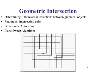
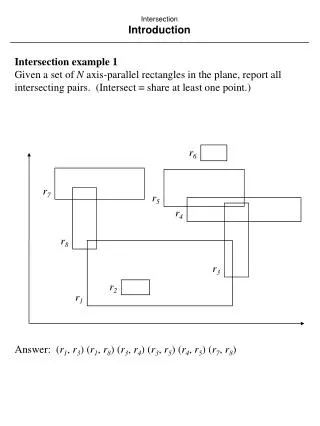
Intersection Introduction. Intersection example 1 Given a set of N axis-parallel rectangles in the plane, report all intersecting pairs. (Intersect share at least one point.). r 6. r 7. r 5. r 4. r 8. r 3. r 2. r 1.

Intersection Introduction
E N D
Presentation Transcript
IntersectionIntroduction Intersection example 1 Given a set of N axis-parallel rectangles in the plane, report all intersecting pairs. (Intersect share at least one point.) r6 r7 r5 r4 r8 r3 r2 r1 Answer: (r1, r3) (r1, r8) (r3, r4) (r3, r5) (r4, r5) (r7, r8)
IntersectionIntroduction Intersection example 2 Given two convex polygons, construct their intersection. (Polygon boundary and interior, intersection all points that are members of both polygons.) A B A B
IntersectionIntroduction General intersection problems Test or decision problem Given two geometric objects, determine if they intersect. Pairwise counting or reporting problem Given a data set of N geometric objects, count or report theirintersections. Construction problem Given a data set of N geometric objects, construct a new object which is their intersection.
IntersectionIntroduction Applications Domain: GraphicsProblem: Hidden-line and hidden surface removalApproach: Intersection of two polygonsType: Construction Domain: Pattern recognitionProblem: Finding a linear classifier between two sets of pointsApproach: Intersection of convex hullsType: Test Domain: VLSI designProblem: Component overlap detectionApproach: Intersection of rectanglesType: Pairwise
IntersectionIntersection of line segments Problem definition Given N line segments in the plane, report all their points of intersection (pairwise). LINE SEGMENT INTERSECTION (LSI). INSTANCE: Set S = {s1, s2, ..., sN} of line segments in the plane. For 1 iN, si = (ei1, ei2) (endpoints of the segments), and for 1 j 2, eij = (xij, yij) (coordinates of the endpoints). QUESTION: Report all points of intersection of segments in S. Note that this problem is single-shot, not repetitive mode. Assumptions 1. No segments of S are vertical. 2. No three segments meet at a point.
IntersectionIntersection of line segments, brute force algorithm Algorithm For every pair of segments in S, test the two segments for intersection. (Segment intersection test can be done in constant time. The test involves the parametric equations of the lines defined by the segments and the dot product operation. See Laszlo pp. 90-93 for details.) Analysis Preprocessing: None Query: O(N2); there are N(N - 1) / 2 O(N2) pairs, each requiring a constant time test. Storage: O(N); for S. Can we do better?
s2 s1 s3 s4 v u IntersectionIntersection of line segments, Shamos-Hoey algorithm Segment ordering, 1 We need some way to order segments in the plane. Two segments are comparable at abscissa x iff a vertical line through x that intersects both of them. Define the relation above at x as follows: segment s1 is above segment s2 at x, written s1 >xs2, if s1 and s2 are comparable at x and the y-coordinate of the intersection of s1 with the vertical line through x is greater than the y-coordinate of the intersection of s2 with that line. In the example, s2 >us4, s1 >vs2, s2 >vs4, and s1 >vs4. Segment s3 is not comparable with any other segment.
IntersectionIntersection of line segments, Shamos-Hoey algorithm Segment ordering, 2 Preparata defines relation >x for “non-intersecting” segments (see p. 281), and then applies it to segments that may intersect (see p. 282). Luckily, this does not affect the algorithm. As the vertical line sweeps, the ordering changes in three ways: 1. The left endpoint of a segment s is encountered. Segment s must be added to the ordering. 2. The right endpoint of a segment s is encountered. Segment s must be removed from the ordering. 3. An intersection point of two segments s1and s2 is encountered. Segments s1and s2, exchange places in the ordering.
IntersectionIntersection of line segments, Shamos-Hoey algorithm Algorithm idea s1 s2 x Crucial observation: For two segments s1and s2 to intersect, there must be some x for which s1and s2 are consecutivein the >x ordering. This suggests that the sequence of intersections of the segments with the vertical line contains the information needed to find the intersections between the segments. That suggests a plane sweep algorithm. Plane sweep algorithms often use two data structures: 1. Sweep-line status 2. Event-point schedule
IntersectionIntersection of line segments, Shamos-Hoey algorithm Sweep-line status The sweep-line status is a list of the currently comparable segments, ordered by the relation >x. The sweep-line status data structure L is used to store the ordering of the currently comparable segments. Because the setof currently comparable segments changes, the data structure forL must support these operations: 1. INSERT(s, L). Insert segment s into the total order in L. 2. DELETE(s, L). Delete segment s from L. 3. ABOVE(s, L). Return the name of the segment immediately above s in the ordering in L. 4. BELOW(s, L). Return the name of the segment immediately below s in the ordering in L. The dictionary data structure (see Preparata pp. 11-13) canperform all of these operations in O(log N) time (or better).
IntersectionIntersection of line segments, Shamos-Hoey algorithm Event-point schedule As the sweep-line is swept from left to right, the set of the currentlycomparable segments and/or their ordering by the relation >xchanges at a finite set of x values; those are known as events. The events for this problem are segment endpoints and segment intersections. The event-point schedule data structure E is used to store events prior to their processing. For E the following operations are needed: 1. MIN(E). Determine the smallest element in E (based on x), return it, and delete it. 2. INSERT(x, E). Insert abscissa x, representing an event, into E. 3. MEMBER(x, E). Determine if abscissa x is a member of E. The priority queue data structure (see Preparata pp. 11-13) canperform all of these operations in O(log N) time.
IntersectionIntersection of line segments, Shamos-Hoey algorithm Algorithm 1 procedure LineSegmentIntersection(S) 2 begin 3 Sort the 2N endpoints of S lexicographcially by x and y and load them into E; 4 A = ; /* A is an internal working queue. */ 5 while (E) do 6 begin 7 p = MIN(E); 8 if (p is a left endpoint) then 9 begin 10 s = segment of which p is endpoint; 11 INSERT(s, L); 12 s1 = ABOVE(s, L); 13 s2 = BELOW(s, L): 14 if (s1 intersects s) then add (s1, s) to A; 15 if (s2 intersects s) then add (s2, s) to A; 16 end 17 else if (p is a right endpoint) then 18 begin 19 s = segment of which p is endpoint; 20 s1 = ABOVE(s, L); 21 s2 = BELOW(s, L): 22 if (s1 intersects s2 to the right of p) then add (s1, s2) to A; 23 DELETE(s, L); 24 end 25 else /* p is an intersection */ 26 begin 27 s1, s2 = segments that intersect at p, with s1 above s2 to the left of p. 28 s3 = ABOVE(s1 , L); 29 s4 = BELOW(s2 , L): 30 if (s3 intersects s2) then add (s3, s2) to A; 31 if (s1 intersects s4) then add (s1, s4) to A; 32 Interchange s1 and s2 in L; 33 end Algorithm continued on next page.
IntersectionIntersection of line segments, Shamos-Hoey algorithm Algorithm, 2 34 /* The detected intersections must now be processed */ 35 while (A) do 36 begin 37 (s1, s2) = get and remove first element of A; 38 x = x-coordinate of intersection point of s1 and s2; 39 if (MEMBER(x, E) = FALSE) then 40 begin 41 report (s1, s2); 42 INSERT(x, E); 43 end 44 end 45 end 46 end The “while (A) do” block (lines 35-44) is within the “while (E) do”begin-end block (lines 5-45).
IntersectionIntersection of line segments, Shamos-Hoey algorithm Problems with the Shamos-Hoey algorithm, as given in Preparata Cases excluded by assumption: 1. Vertical segments. 2. Three (or more) segments intersecting at a single point. Cases not handled: 1. Multiple intersections at same abscissa (fails at line 39).2. Intersection and endpoint at same abscissa (fails at line 39). 3. Segments that intersect at endpoints (special case of 2, pointed out by Franceschini).4. Segments that intersect at >1 point (i.e. collinear overlap).5. Event type (left endpoint, right endpoint, intersection) is tested by the algorithm (lines 8 and 17) but never stored in E. 1 2 3 4
IntersectionIntersection of line segments, Shamos-Hoey algorithm Analysis Preprocessing: O(N log N); sort of endpoints.Query: O((N + K) log N); each of 2N endpoints and K intersections are inserted into E, an O(log N) operation.Storage: O(N + K); at most 2N endpoints and K intersections arestored in E. Comments Here “query” refers to the process of finding intersections; this is a single-shot problem. Query time of O((N + K) log N) is suboptimum. An optimum O(N log N + K) algorithm exists, but is quite difficult. Laszlo (1996) still presents the Shamos-Hoey algorithm (1976) 20 years later.
IntersectionInterval trees Notation The notation used here for interval trees is not consistent with eitherPreparata (pp. 359-363) or Ullman (pp. 385-393), which areunfortunately not consistent with each other.This notation is consistent with notation used earlier for similar concepts regarding segment trees. Definition, 1 An interval tree is a rooted binary tree that stores data intervals onthe real line whose endpoints are integers within a fixed scope. It is the scope from within the endpoints are chosen that is fixed, not the data interval endpoints themselves. The tree structure in which the intervals are stored is defined for a scope interval [l, r], where l and r must be consecutive multiplesof the same power of 2.For a given [l, r] there is exactly one interval tree structure.The data intervals are stored within the fixed tree.We will assume WLOG that the data interval endpoints havebeen normalized to [1, N] and the tree has been built for scopeinterval [0, 2k], where N + 1 2k. T(l, r) = Interval tree over scope interval [l, r]. Each node of T(l, r) is associated with a scope interval [l, r].
IntersectionInterval trees Definition, 2 A node v has these parameters: B(v) Beginning of scope interval associated with this node. E(v) End of scope interval associated with this node.M(v) Midpoint of scope interval, M(v) = (B(v) + E(v)) / 2 Lchild(v) Left subtree = T(B(v), (B(v) + E(v)) / 2) Rchild(v) Right subtree = T((B(v) + E(v)) / 2E(v)) L(v) AVL tree containing data intervals stored at v, ordered on ascending left endpoint.R(v) AVL tree containing data intervals stored at v, ordered on descending right endpoint.Lptr(v) Pointer to left subchild in secondary search tree.Rptr(v) Pointer to right subchild in secondary search tree. Status(v) { active, inactive } = active iff (L(v) or there are active nodes in both subtrees (Lchild(v) and Rchild(v)) [B(v), E(v)] is the scope interval associated with node v. We will refer to a data interval as [b, e]. Data intervals will bestored at the highest node where B(v) < bM(v) e < E(v). Operations preview. The interval tree supports interval insert, delete, and queryoperations, all in O(log N) time, as will be shown. Query is defined as reporting overlaps between a query interval and the data intervals stored in the tree.
IntersectionInterval trees Example The structure of the interval tree T(0,16) is shown; 0 = 0 · 24, 16 = 1 · 24. Each node is labeled with B(v), E(v) of its scope interval. 0,16 [7,12] 0,8 8,16 [0,4] [1,6] 0,4 4,8 8,12 12,16 [9,10] [6,7] [13,15] [9,11] 0,2 2,4 4,6 6,8 8,10 10,12 12,14 14,16 [1,1] Data intervals [0,4], [7,12], [9,10], [9,11], [1,1], [6,7], [13,15],and [1,6] are shown below the node where they would be stored. Note that T(0,16) is shown here down to a level that accomodates 0 length intervals (e.g. [1,1]); if such degenerate cases will not occur, the lowest level is usually not represented. To simplify the figures, that level (and interval [1,1]) will be omitted hereinafter.
0,16 [7,12] 0,8 8,16 0,4 4,8 8,12 12,16 [6,7] [9,10] [13,15] [9,11] L R [0,4] [1,6] [1,6] [0,4] IntersectionInterval trees Data trees Each node v has attached two AVL trees, L(v) and R(v), that hold the intervals stored at this node, ordered by ascending left endpoint and descending right endpoint respectively. L(v) and R(v) are shown for node 0,8 only; every node would have similar trees. ascending left descending right L(v) and R(v) are threaded to allow ordered scans of the data intervals contained therein without requiring a binary search.
0,16 [7,12] 0,8 8,16 0,4 4,8 8,12 12,16 [9,10] [6,7] [13,15] [9,11] IntersectionInterval trees Secondary search tree The active nodes of an interval tree are connected by pointers, forming a secondary binary search tree within the interval tree. The secondary search tree allows the interval tree to be searched without requring numerous accesses to empty nodes. Lptr(v) and Rptr(v) hold the secondary search tree pointers. Active nodes are in the secondary search tree. In this example, data intervals [0,4] and [1,6] are not present. Nodes 0,16, 4,8, 8,12, and 12,16 are active because there aredata intervals stored at those nodes. Node 8,16 is active because both of its child nodes are active. Nodes 0,8 and 0,4 are inactive because there are no intervals stored at those nodes and neither has two active child nodes. Because a binary tree has one more leaf node than internal nodes, it can be shown that the number of empty active nodes is lessthan half the number of non-empty active nodes.
IntersectionInterval trees Insertion The interval tree T(l,r) supports insertions and deletions of data intervals [b, e] with endpoints l < be < r,in O(log N) time per operation. As mentioned, data interval [b, e] inserted into T(l, r)will be stored at the highest node where bM(v) e. To insert interval [b, e] into interval tree T(l,r): InsertIntervalTree(b, e, root(T)) procedure InsertIntervalTree(b, e, v) begin if (bM(v) e) then /* Data interval straddles midpoint */ add [b, e] to L(v) and R(v) /* 2 O(log N) */ adjust the secondary search tree pointers as needed else if (eM(v)) then /* Data interval left of midpoint */ InsertIntervalTree(b, e, Lchild(v)) else /* M(v) b, Data interval right of midpoint */ InsertIntervalTree(b, e, Rchild(v)) end end
IntersectionInterval trees Deletion Deletion is symmetric with insertion. To delete interval [b, e] from interval tree T(l,r): DeleteIntervalTree(b, e, root(T)) procedure DeleteIntervalTree(b, e, v) begin if (bM(v) e) then delete [b, e] from L(v) and R(v) /* 2 O(log N) */ adjust the secondary search tree pointers as needed else if (eM(v)) then DeleteIntervalTree(b, e, Lchild(v)) else /* M(v) b */ DeleteIntervalTree(b, e, Rchild(v)) end end
IntersectionInterval trees Query To report data intervals that overlap query interval [b, e]: QueryIntervalTree(b, e, root(T)) procedure QueryIntervalTree(b, e, v) begin if (bM(v) e) then /* Query interval straddles midpoint, as do all intervals at v */ begin report all intervals in L(v) QueryIntervalTree(b, e, Lptr(v)) QueryIntervalTree(b, e, Rptr(v)) end else if (eM(v)) then /* Query interval to left of midpoint */ begini = 1 while (the ith interval [li, ri] in L(v) has lie) do begin report [li, ri] i++ end QueryIntervalTree(b, e, Lptr(v)) end else /* M(v) b, i.e. query interval to right of midpoint */ begini = 1 while (the ith interval [li, ri] in R(v) has rib) do begin report [li, ri] i++ end QueryIntervalTree(b, e, Rptr(v)) end endend Note that Lptr(v) and Rptr(v) are used (not Lchild(v) and Rchild(v))so as to use the secondary search tree.
IntersectionInterval trees Analysis preliminaries It must be shown that the query algorithm has time complexity O(log N + K). reporting overlaps traversal time To do so, it will be necessary to consider the interval tree data structure and the geometric interpretation of the data simultaneously. Recall that the query traverses the secondary search tree, rather than the primary interval tree, thereby bypassing inactive nodes. Scope interval Interval represented by a node; [B(v), E(v)].Data interval Interval stored at a node; by definition, straddles the midpoint M(v) of the scope interval.Query interval Interval against which the data intervals are being compared for overlap; [b, e].
b e b e A or B(v) M(v) E(v) B(v) M(v) E(v) b e B B(v) M(v) E(v) b e b e C1 or B(v) M(v) E(v) B(v) M(v) E(v) b e e b C2 or B(v) M(v) E(v) B(v) M(v) E(v) b e D B(v) M(v) E(v) IntersectionInterval trees Overlap classes During a query traversal, the “overlap” between a query interval[b, e] and a scope interval [B(v), E(v)] for a node will be one offive classes:
IntersectionInterval trees Transition rules for overlap classes As the query traversal proceeds, the overlap class at a node determines the type(s) of overlap classes that can occur at the descendants of that node later/lower in the traversal. ClassClass of Left ChildClass of Right Child A A or B* No intersection* B C1 or C2 C1 or C2 C1 D C1 or C2 C2 C1 or C2* No intersection* D D D * These entries assume left overlap; they are reversed forright overlap.
D D IntersectionInterval trees Overlap classes for a query traversal The overlap transition rules mean that tree traversed by a query will look something like this. (This is the table from the previous page arranged as a tree.) A A B C C C D C C C C C C = C1 or C2 Once a class D node is reached, all data intervals in the subtreeoverlap the query interval and will be reported.
IntersectionInterval trees Traversal length, 1 The overlap transition rules imply a maximum “fan out” of the tree searched in a query traversal. Number ofNumber of non-DClassChild Nodes to SearchChild Nodes to Search A 1 1 B 1 or 2 1 or 2 C1 or C2 1 or 2 1 D 2 0 No A, B, or C (C1 or C2) node requires the search of > 2 child nodes. The secondary search tree has depth log N. The number of class A, B, or C nodes traversed in a query is 2 log N.The query time complexity, neglecting class D nodes, is O(log N). But what about class D nodes?
IntersectionInterval trees Traversal length, 2 Close but not quite right answer: Every data interval at a class D node overlaps the query interval. The time to access the class D nodes can be charged to reporting, i.e. is O(K). This is not quite right because some active class D nodes mighthave empty data interval lists; they are active because both subtreesare active. Right answer: A binary tree has one more leaf the non-leaf nodes.The subtrees of the class D nodes are binary trees.More than half of the class D nodes have non-empty interval lists. The time to access the class D nodes, both empty and non-empty, can be charged to reporting, i.e. is O(K). Overall query time complexity O(log N + K); O(log N) to traverse the class A, B, C1, and C2 nodes, and O(K) to traverse the class D nodes and report overlappingintervals.
IntersectionInterval trees Storage analysis Assume N data intervals. 2N distinct endpoints after normalization. 2k-1 2N 2kUpper limit 2k because for T(l,r) r must be a multiple of a power of 2.Lower limit 2k-1 because otherwise 2k-1 would be r.2k-1) 2(2N) 2(2k) Multiply through by 2. 2k 4N 2k+1 2N 2k 4N Collect terms.2kO(N) Primary interval tree has O(N) nodes and O(log N) levels. There are a total of 2N intervals stored in the data trees attached tothe nodes. (A data interval is stored at one node in an interval tree, in the L and R AVL trees at that node.)
IntersectionInterval trees Analysis summary Preprocessing: O(N log N); N data intervals, O(log N) to insert each. There are actually 3 O(log N) operations per insertions: (1) traversing the primary search tree (2) inserting the data interval into L AVL tree (3) inserting the data interval into R AVL treeQuery: O(log N + K); as shown.Storage: O(N); as shown. Comments Observe that the data trees need to be AVL trees only if O(log N) insert and delete operations are needed. If the data set is static,simple lists can be used instead, because the query operation scans the data lists anyway. The interval tree is a versatile data structure. We will use it to solve the next intersection problem.
(xil, yir) (xir, yir) ri (xil, yil) (xir, yil) Considered to intersect. IntersectionIntersection of rectangles Problem definition RECTANGLE INTERSECTION INSTANCE: Set S = {r1, r2, ..., rN} of rectangles in the plane. For 1 iN, ri = ((xil, yil), (xil, yir), (xir, yil), (xir, yir)). QUESTION: Report all pairs of rectangles that intersect. (Edge and interior intersections should be reported.) Note that is is a single-shot, rather than repetitive mode, problem.
r6 r7 r5 r4 r8 r3 r2 r1 r9 Answer: (r1, r3) (r1, r8) (r3, r4) (r3, r5) (r4, r5) (r7, r8) (r1, r2) (r3, r9) IntersectionIntersection of rectangles
IntersectionIntersection of rectangles Brute force algorithm For every pair (ri, rj) of rectangles S, ij if (rirj ) then report (ri, rj) Analysis Preprocessing: None. Query: O(N2); N = (N(N - 1))/2 O(N2). 2Storage: O(N). ( )
r6 r7 r5 r4 r8 r3 r2 r1 r9 Answer: (r1, r3) (r1, r8) (r3, r4) (r3, r5) (r4, r5) (r7, r8) (r1, r2) (r3, r9) IntersectionIntersection of rectangles Algorithm using interval trees Plane sweep algorithm, vertical sweep line from left to right. Event points are left and right edges of rectangles. At left edge: 1. Compare rectangle y-interval to active set for overlap. 2. Add rectangle y-interval to active set.At right edge: Remove rectangle y-interval from active set. Active set maintained in interval tree.
IntersectionIntersection of rectangles N, N, what is N? N rectangles in S 4N distinct coordinates for vertices: xil, xir, yil, yir for 1 iN. Assume x- and y-coordinates are normalized together as [1,4N]. Interval tree T(l,r) is built for scope interval [0,2k]. 0 1 4N 4N + 1 2k Smallest (normalized) coordinate Smallest power of 2 2k 4N + 1 Left end of interval tree scope interval Right end of interval tree scope interval Largest (normalized) coordinate Number of nodes and depth of tree dependent on 2k, not N? Can operation time complexity be expressed as function of N? 2k-1 4N + 1 2kUpper limit 2kby choice (smallest power of 2 2k 4N + 1).Lower limit 2k-1 because otherwise 2k-1 would be upper limit.2k-1) 2(4N + 1) 2(2k) Multiply through by 2. 2k 8N + 2 2k+1 4N + 1 2k 8N + 2 Collect terms.2kO(N) Primary interval tree has O(N) nodes and O(log N) levels.
IntersectionIntersection of rectangles Preprocessing Normalize x- and y-coordinates of rectangles. O(N log N) for sort.Construct (empty) interval tree T(0,2k). O(N) (The interval tree is the sweep-line status.) Initialize event queue Q with rectangle vertical edges:(xil, yil, yir, left) and (xir, yil, yir, right) for 1 iN,in ascending x order, and for edges with the same x, left edges ahead of right. O(N), read off after sort. Query while (Q) dobegin Get next entry (xil, yil, yir, t) from Q /* t {left, right} */ if t = left then begin /* left edge */ QueryIntervalTree(yil, yir, root(T)) InsertIntervalTree(yil, yir, root(T)) end else /* right edge */ DeleteIntervalTree(yil, yir, root(T))end For a left edge, the query precedes the insert to avoid reporting overlap with self. For multiple edges with the same x-coordinate, left edges aresorted ahead of right so as to find edge-only intersections.
IntersectionIntersection of rectangles Analysis Preprocessing: O(N log N); as shown. Query: O(N log N + K); O(N) edges, O(log N) for each. Storage: O(N); interval tree O(N) as shown,event queue also O(N). Comments Here “Query” refers to the process of finding the intersections; this is a single-shot problem. O(N log N + K) is lower bound for rectangle intersection problem. Can be shown by lower bounds proof. We’ve gone to a lot of trouble to improve the time from O(N2) to O(N log N), i.e., interval tree. Difference between O(N2) and O(N log N) is significant for VLSI applications; e.g. if N = 106, N2 = 1012 and N log N = 2 107.
IntersectionIntersection of convex polygons Problem descriptionHere we consider a category of related intersection constructionproblems: Given two (or more) geometric objects, constructa new object which is their intersection. The objects dealt with will be polygons, polyhedra, half-planes, half-spaces, and related types. The objects will generally be specified by their vertices and orientations to identify the interior of the object. (The latter may be given by convention.) Applications. Graphics, constructive solid modeling, linear programming.
IntersectionIntersection of convex polygons Intersection of arbitrary polygonsThe intersection of two arbitrary polygons can have quadratic complexity. The intersection shown below consists of 25 squares.
q1 p1 pN p2 q2 qM p3 q3 p8 P R Q q4 p4 q7 p7 q5 p5 q6 p6 IntersectionIntersection of convex polygons Problem definitionFor convex (rather than arbitrary) polygons, problem is linear. CONVEX POLYGON INTERSECTION. INSTANCE: Convex polygons P and Q, with vertex sets P = {p1, p2, ..., pN} and Q = {q1, q2, ..., qM} respectively.QUESTION: Construct polygon R which is their intersection. The intersection of two convex polygons will have linear O(N + M) complexity (both the object and the construction process). By convention, P, Q, and R will be oriented counterclockwise, so that the interiors of the polygons lie to the left of their edges (as in Preparata and Laszlo, opposite of O’Rourke).
IntersectionIntersection of convex polygons O’Rourke-Chien-Olson-Naddor algorithmThis same algorithm described in three sources:1. O’Rourke, section 7.4, pp. 243-252, with C code.2. Preparata, pp. 273-277.3. Laszlo, section 6.5, pp. 154-162, with C++ code. Presentation is a synthesis of all three. Notation of sources inconsistent, Preparata used primarily. Exposition of sources inconsistent, Laszlo used primarily. The algorithm is based on three undergraduates’ homework assignment solutions in 1982. Simpler than previously existing linear O(N + M) algorithm, e.g., Shamos’ 1978 algorithm.
IntersectionIntersection of convex polygons Intersection structureThe objective is to form the intersection polygon R of two convex polygons P and Q. For the moment, assume that the edges of P and Q intersect non-degenerately; when two edges intersect, they do so at a single point. Given this assumption, the boundary of R = PQ consists of alternating chains of vertices from P and Q. Consecutive chains are joined at intersection points, where an edge of P intersects an edge of Q. Intersection point P Q Chain from P Chain from Q In fact, the algorithm will handle degenerate intersections.
IntersectionIntersection of convex polygons Sickles, 1Regions that are within one polygon, but not both, are called sickles. Sickles are bounded by two chains (inner and outer) of vertices, one from each polygon, and terminated by intersection pointsat either end. The boundary of PQ is formed from the inner chains of the sickles. Outer chain Initial intersection point Inner chain Terminal intersection point
IntersectionIntersection of convex polygons Sickles, 2A vertex (of P or Q) belongs to a sickle either if: 1. It lies between the initial and terminal intersection points on either chain.2. It is the destination of the edge of the internal chain containing the terminal intersection point of the sickle. Note that some vertices may belong to > 1 sickles. Initial intersection point Terminal intersection point Also belongs to next sickle
IntersectionIntersection of convex polygons Algorithm overview, 1Define current edges of P and Q: edge(pi-1pi) and edge(qj-1qj), with destinations pi and qj, respectively. p0 = pN and q0 = qM, by definition. IntersectConvexPolygons(P, Q) /* Informal */ begin i = j = 1 /* Arbitrarily start with vertex 1 of each polygon. */ repeat if ((w = edge(pi-1pi) edge(qj-1qj)) ) then add w to RSelect current edge to advance based on configuration. if (selected edge is on inner chain) then begin add selected edge destination to R increment index of selected edge end until iterations > 3(N + M) /* Preparata erroneously says 2 */ if (R = ) then /* Boundaries of P and Q don’t intersect */ resolve special cases PQ, QP, PQ = end
IntersectionIntersection of convex polygons Algorithm overview, 2The algorithm has two phases, both handled by same advance rules: 1. Get current edges edge(pi-1pi) and edge(qj-1qj) into same sickle.2. Advance current edges edge(pi-1pi) and edge(qj-1qj) together through each sickle, adding inner chain vertices to R; and advance them both into the next sickle. Before either leaves the current sickle for the next sickle the terminal intersection point will be found.
IntersectionIntersection of convex polygons Aiming atAdvance rules are used to select the current edge to advance. The advance rules depend on the notion of “aiming at”. The bold arrows aim at edge(qj-1qj). qi-1 qi If they are not collinear,edge(pi-1pi) aims at edge(qj-1qj) if either of these conditions hold: 1. edge(pi-1pi) edge(qj-1qj) 0 andpi does not lie to the right of edge(qj-1qj).2. edge(pi-1pi) edge(qj-1qj) < 0 andpi does not lie to the left of edge(qj-1qj). If they are collinear,edge(pi-1pi) aims at edge(qj-1qj) if pi does not lie beyond qj.
IntersectionIntersection of convex polygons Advance rules, overall intentAdvance rules are used to select the current edge to advance. O’Rourke: ‘If edge(pi-1pi) aims at the line containing edge(qj-1qj) but does not cross it, we want to advance edge(pi-1pi) to close in on a possible intersection point with edge(qj-1qj).’ Laszlo: ‘The advance rules are designed so that the intersection point which should be found next is not skipped over. They distinguish between the current edge which may contain the next intersection point and the current edge which cannot possibly contain the next intersection point; the latter edge is advanced.’ Preparata: ‘The idea is to not advance on the boundary (either of P or of Q) whose current edge may contain a yet to be found intersectionpoint.’
IntersectionIntersection of convex polygons Advance rules, Preparata and Laszlo: Case (1) qj pi qj pi Advance Advance Preparata Laszlo Laszlo: Edge(pi-1pi) and edge(qj-1qj) aim at each other:Advance whichever edge is to the right of the other. (assuming CCW orientation for P and Q).Assume edge(qj-1qj) is to the right; then the next intersection pointcannot lie on edge(qj-1qj) because qj is outside the intersectionpolygon R. Preparata: The choice is arbitrary, and we elect to advance on edge(qj-1qj).