Download
1 / 13
170 likes | 364 Vues
Introduction to Basic Inventory Control Theory. Topics Covered. Problem Definition: When and How much to order The EOQ formula: underlying modeling assumptions and derivation The geometric interpretation of the EOQ formula and its implications for the model robustness

E N D
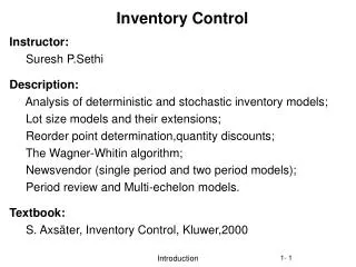
Topics Covered • Problem Definition: When and How much to order • The EOQ formula: underlying modeling assumptions and derivation • The geometric interpretation of the EOQ formula and its implications for the model robustness • Introducing buffering capacity constraints • Re-order point for deterministic non-zero lead times • Production Order Quantity (POQ) model • Optimal order quantity under quantity discounts: The all-units discount case • Probabilistic models with constant lead time • System Integration: Continuous vs Periodic review models • Paretto Law and ABC analysis
Main Issues to be addressed • When to order for replenishment? • How much to order? • Two major classes of policies • Continuous review policies • Periodic review policies
The basic EOQ Model • Model Assumptions: • Deterministic demand rate: D (units / yr) • Infinite Operational Horizon • Continuous Review • Instantaneous Replenishment IP Q D time T Need to minimize annual total cost w.r.t. Q: TAC(Q) = Item-AC(Q) + Ordering-AC(Q)+Holding-AC(Q) = C($/unit)*D(units/yr) + S($/order) *D(units/yr) / Q(units/order) + H($/unit x yr)*[Q*T / 2](units x yr / order)*[1/T](orders/yr) dTAC(Q)/dQ = 0 => Q* = [ 2*S*D / H]1/2
A geometric interpretation of the EOQ formula and its implications Cost SD/Q+HQ/2 HQ/2 SD/Q Q Q* • Implications: • Under finite buffering/storage capacity Qstor, the optimum order • size is Q*, if Qstor Q*, and Qstor otherwise. • It can be shown that the cumulative curve is quite flat around its • minimum, and therefore, picking an order size that is different from • but fairly close to Q* does not alter significantly the annual total cost. • What is the practical significance of item 2 above?
Variations of the EOQ Model • Deterministic non-zero lead time: L (yrs) => • Reorder Point (ROP) = L(yrs)* D(units/yrs) • Production Order Quantity Model: • Finite Production Rate, P (units/yr) IP Q-D(Q/P) P-D D time TAC(Q) = Item-AC(Q) + Ordering-AC(Q)+Holding-AC(Q) = C($/unit)*D(units/yr) + S($/order) *D(units/yr) / Q(units/order) + H($/unit x yr)*[Q*(1-D/P)*T / 2](units x yr order)*[1/T](orders/yr) => Q* = [ 2*S*D / (H*(1-D/P))]1/2
Application of the EOQ theory under total quantity discounts • Suppose that the unit purchasing cost C depends on the ordered quantity, Q. In particular, C obtains a certain value, C1, if Q lies in the interval (0,Q1], C2, if Q lies in the interval (Q1,Q2], …, Cn, if Q lies in the interval (Qn-1,Qn], and Cn+1, if Q lies in the interval (Qn,). Furthermore, C1 > C2 > …> Cn > Cn+1. • Then, letting • ATC(i)(Q)= Ci*Q+S*D/Q + H(Ci)*Q/2 • where • H(Ci) = I*Ci and I is the applying interest rate, • We obtain the following graphical representation for the curves ATC(i)(Q) and • ATC(Q): ATC ATC(1) ATC(i) ATC(n+1) Q Q1 Qi-1 Qi Qn
Application of the EOQ theory under total quantity discounts • The previous plot suggests the following algorithm for computing the EOQ under total quantity discounts: • For each curve TAC(i)(Q) compute the quantity Q(i) that minimizes TAC over that curve; this can be done as follows: • Compute Q*(i) according to the standard EOQ formula while using Ci in the evaluation of H(Ci). • If Q*(i) belongs in the application interval for TAC(i)(Q), then set Q(i) = Q*(i) (since Q*(i) is a feasible point). • If Q*(i) lies to the left of the application interval for TAC(i)(Q), then set Q(i) = minimum of the application interval for TAC(i)(Q). • If Q*(i) lies to the right of the application interval for TAC(i)(Q), then set Q(i) = maximum of the application interval for TAC(i)(Q). • For each selected Q(i), compute the corresponding TAC(i)(Q(i)), and pick a Q(i), that provides the smallest TAC(i)(Q(i)) value. • Remark: A more efficient implementation of the above algorithm is as follows: • Start the above computations from TAC(n+1)(Q(n+1)), and carry them on in decreasing order of i, until you exhaust all i’s, or you find an interval for which Q(i) = Q*(i). In the latter case, you can ignore all the remaining i’s.
A continuous review model with probabilistic demand and constant lead time • Model Assumptions: • Stochastic demand rate; in particular, daily demand is a random • variable (r.v.) dd N(Dd, d2). • Infinite Operational Horizon • Continuous Review • Lead time is deterministic; in particular L days. • Then, • The expected TAC is minimized by Q* = [2*S*Da/H]1/2, where • Da = Dd * (business days in a year). • However, setting ROP = L*Dd, will result in 50% probability of • experiencing a stock-out during every cycle! • To see this, notice that the demand experienced over L days is • another r.v. dL= dd(1)+dd(2)+…+dd(L), and therefore, dLN(L*Dd, • L* d2).
A continuous review model with probabilistic demand and constant lead time • Typically, we want to reduce the probability of stockout during a single replenishment cycle to a value equal to 1-a, where a(0.5,1.0) is known as the desired service level. • This effect can be achieved by setting ROP = L*Dd+ss, where ss is known as the required safety stock. • ss can be computed by solving the following inequality: Prob{dL L*Dd+ss} a Prob{(dL-L*Dd) / (d*L) ss / (d*L)} a ss / (d*L) za where za is the a-th percentile of the standardized normal distribution. • Hence, ROP = L*Dd + za* d*L
Periodic Review Policies • In the case of periodic review policies, we fix the reorder interval T, and every time we place a replenishment order, we check the current inventory position (IP), and order enough to bring this position up to a pre-specified level S. • T is frequently determined by external factors like the supplier delivery schedules. In case of choice, an optimized selection of T is T* = round(Q* / Dd) where Dd is the expected daily demand, Q* = [2*S*Da/H]1/2, and Da = Dd * (business days in a year). • Furthermore, an analysis similar to that provided in the previous two slides, establishes that the minimal re-order level S* that guarantees a service level a, is: S* = T**Dd+za* d*T*, where za and d have the meanings defined in the previous slides. • Remark: Notice that periodic review policies will tend to carry more safety stock than continuous review policies, when applied on the same system, since, in general, T*>L. This is the price of “convenience” provided by these policies, compared to their continuous review counterparts.
The Paretto Effect and ABC Analysis • The Paretto effect can be stated as follows: In a phenomenon that is the cumulative effect of many factors, the largest part of the net result (probably the 80% of it) can be attributed to only a small number of the contributing factors (probably the 20%). • In the case of multi-item inventory systems, this effect manifests itself through the fact that about 80% of the annual total cost is incurred by about 20% of the stored items. • Hence, it is pertinent to characterize the contribution of each item to the annual cost as a percentage of the latter, and then classify the most expensive (about 20%) of these items as class A, the moderately expensive (about 30%) items as class B, and the remaining rather inexpensive items (about 50%) as class C. • Subsequently, tight (typically, continuous review) inventory control must be applied to class A, more relaxed (e.g., periodic review) inventory control may be appropriate for class B, while, for class C, ensuring no sock-outs through over-stocking can be a reasonable / viable approach.
Reading Assignment • Material Presented in class – c.f. your class notes! • From your textbook: • Chapter 4: Sections 4.1-4.7, 4.10 • Chapter 5: 5.1, 5.2, 5.7, 5.9