R and H adoop I ntegrated P rocessing E nvironment
R and H adoop I ntegrated P rocessing E nvironment. Using RHIPE for Data Management. R and Large Data. .Rdata format is poor for large/many objects attach loads all variables in memory No metadata Interfaces to large data formats HDF5, NetCDF.


R and H adoop I ntegrated P rocessing E nvironment
E N D
Presentation Transcript
R and Hadoop Integrated Processing Environment Using RHIPE for Data Management
R and Large Data • .Rdata format is poor for large/many objects • attach loads all variables in memory • No metadata • Interfaces to large data formats • HDF5, NetCDF To compute with large data we need well designed storage formats
R and HPC • Plenty of options • On a single computer: snow, rmpi, multicore • Across a cluster: snow, rmpi, rsge • Data must be in memory, distributes computation across nodes • Needs separate infrastructure for balancing and recovery • Computation not aware of the location of the data
Computing With Data • Scenario: • Data can be divided into subsets • Compute across subsets • Produce side effects (displays) for subsets • Combine results • Not enough to store files across a distributed file system (NFS, LustreFS, GFS etc) • The compute environment must consider the cost of network access
Using Hadoop DFS to Store • Open source implementation of Google FS • Distributed file system across computers • Files are divided into blocks, replicated and stored across the cluster • Clients need not be aware of the striping • Targets write once ,read many – high throughput reads
client File Namenode Blocks Block 1 Block 2 Block 3 Replication Datanode 1 Datanode 2 Datanode 3
Mapreduce • One approach to programming with large data • Powerful tapply • tapply(x, fac, g) • Apply g to rows of x which correspond to unique levels of fac • Can do much more, works on gigabytes of data and across computers
Mapreduce in R If R could, it would: Map: imd <- lapply(input,function(j) list(key=K1(j), value=V1(j))) keys <- lapply(imd,"[[",1) values <- lapply(imd, "[[",2) Reduce: tapply(values,keys, function(k,v) list(key=K1(k,v), value=V1(v,k)))
File Divide into Records of K V pairs Divide into Records of K V pairs Divide into Records of K V pairs For each record, return key, value For each record, return key, value For each record, return key, value Map Sort Shuffle For every KEY reduce K,V For every KEY reduce K,V For every KEY reduce K,V Reduce Write K,V to disk Write K,V to disk Write K,V to disk
R and Hadoop • Manipulate large data sets using Mapreduce in the R language • Though not native Java, still relatively fast • Can write and save a variety of R objects • Atomic vectors,lists and attributes • … data frames, factors etc.
Everything is a key-value pair • Keys need not be unique Block • Run user setup R expression • For key-value pairs in block: • run user R map expression • Each block is a task • Tasks are run in parallel (# is configurable) Reducer • Run user setup R expression • For every key: • while new value exists: • get new value • do something • Each reducer iterates through keys • Reducers run in parallel
Airline Data • Flight information of every flight for 11 years • ~ 12 Gb of data, 120MN rows 1987,10,29,4,1644,1558,1833,1750,PS,1892,NA,109,112,NA,43,46,SEA,..
Save Airline as R Data Frames 1. Some setup code, run once every block of e.g. 128MB (Hadoop block size) setup <- expression({ convertHHMM <- function(s){ t(sapply(s,function(r){ l=nchar(r) if(l==4) c(substr(r,1,2),substr(r,3,4)) else if(l==3) c(substr(r,1,1),substr(r,2,3)) else c('0','0') }) )} })
Save Airline as R Data Frames 2. Read lines and store N rows as data frames map <- expression({ y <- do.call("rbind",lapply(map.values,function(r){ if(substr(r,1,4)!='Year') strsplit(r,",")[[1]] })) mu <- rep(1,nrow(y)) yr <- y[,1]; mn=y[,2];dy=y[,3] hr <- convertHHMM(y[,5]) depart <- ISOdatetime(year=yr,month=mn,day=dy,hour=hr[,1],min=hr[,2],sec=mu) .... .... Cont’d
Save Airline as R Data Frames 2. Read lines and store N rows as data frames map <- expression({ .... From previous page .... d <- data.frame(depart= depart,sdepart = sdepart ,arrive = arrive,sarrive =sarrive ,carrier = y[,9],origin = y[,17] ,dest=y[,18],dist = y[,19] ,cancelled=y[,22], stringsAsFactors=FALSE) rhcollect(map.keys[[1]],d) }) Key is irrelevant for us Cont’d
Save Airline as R Data Frames 3. Run z <- rhmr(map=map,setup=setup,inout=c("text","sequence") ,ifolder="/air/",ofolder="/airline") rhex(z)
Quantile Plot of Delay • 120MN delay times • Display 1K quantiles • For discrete data, quite possible to calculate exact quantiles • Frequency table of distinct delay values • Sort on delay value and get quantile
Quantile Plot of Delay map <- expression({ r <- do.call("rbind",map.values) delay <- as.vector(r[,'arrive'])-as.vector(r[,'sarrive']) delay <- delay[delay >= 0] unq <- table(delay) for(n in names(unq)) rhcollect(as.numeric(n),unq[n]) }) reduce <- expression( pre = { summ <- 0 }, reduce = { summ <- sum(summ,unlist(reduce.values)) }, post = { rhcollect(reduce.key,summ) } )
Quantile Plot of Delay • Run z=rhmr(map=map, reduce=reduce,ifolder="/airline/",ofolder='/tmp/f' ,inout=c('sequence','sequence'),combiner=TRUE ,mapred=list(rhipe_map_buff_size=5)) rhex(z) • Read in results and save as data frame res <- rhread("/tmp/f",doloc=FALSE) tb <- data.frame(delay=unlist(lapply(res,"[[",1)) ,freq = unlist(lapply(res,"[[",2)))
Conditioning • Can create the panels, but need to stitch them together • Small change … map <- expression({ r <- do.call("rbind",map.values) r$delay <- as.vector(r[,'arrive'])-as.vector(r[,'sarrive']) r-r[r$delay>=0,,drop=FALSE] r$cond <- r[,'dest'] mu <- split(r$delay, r$cond) for(dst in names(mu)){ unq <- table(mu[[dst]]) for(n in names(unq)) rhcollect(list(dst,as.numeric(n)),unq[n]) } })
Conditioning • After reading in the data (list of lists) list( list(“ABE”,7980),15) • We can get a table, ready for display dest delay freq 1 ABE 7980 15 2 ABE 61800 4 3 ABE 35280 5 4 ABE 56160 1
Running a FF Design • Have an algorithm to detect keystrokes in a SSH TCP/IP flow • Accepts 8 tuning parameters, what are the optimal values? • Each parameter has 3 levels, construct a 3^(8-3) FF design which spans design space • 243 trials, each trial an application of algorithm to 1817 connections (for a given set of parameters)
Running an FF Design • 1809 connections in 94MB • 439,587 algorithm applications Approaches • Each connection run 243 times? (1809 in parallel) • Slow, running time is heavily skewed • Better: chunk 439,587
Chunk == 1, send data to reducers m2 <- expression({ lapply(seq_along(map.keys),function(r){ key <- map.keys[[r]] value <- map.values[[r]] apply(para3.r,1,function(j){ rhcollect(list(k=key,p=j), value) }) }) }) • map.values is a list of connection data • map.keys are connection identifiers • para3.r is list of 243 parameter sets
Reduce: apply algorithm r2 <- expression( reduce={ value <- reduce.values[[1]]; params <- as.list(reduce.key$p) tt=system.time(v <- ks.detect(value,debug=F,params=params ,dorules=FALSE)) rhcounter('param','_all_',1) rhcollect(unlist(params) ,list(hash=reduce.key$k,numks=v$numks, time=tt)) }) • rhcounter updates “counters” visible on Jobtracker website and returned to R as a list
FF Design … cont’d • Sequential running time: 80 days • Across 72 cores: ~32 hrs • Across 320 cores(EC2 cluster, 80 c1.medium instances): 6.5 hrs ($100) • A smarter chunk size would improve performance
FF Design … cont’d • Catch: Map transforms 95MB into 3.5GB! (37X). • Soln: Use Fair Scheduler and submit(rhex) 243 separate MapReduce jobs. Each is just a map • Upon completion: One more MapReduce to combine the results. • Will utilize all cores and save on data transfer • Problem: RHIPE can launch MapReduce jobs asynchronously, but cannot wait on their completion
Large Data • Now we have 1.2MN connections across 140GB of data • Stored as ~1.4MN R data frames • Each connection as multiple data frames of 10K packets • Apply algorithm to each connection m2 <- expression({ params <- unserialize(charToRaw(Sys.getenv("myparams"))) lapply(seq_along(map.keys),function(r){ key <- map.keys[[r]] value <- map.values[[r]] v=ks.detect(value,debug=F,params=params,dorules=FALSE) ….
Large Data • Can’t apply algorithm to huge connections – takes forever to load in memory • For each of 1.2 MN connections, save 1st (time) 1500 packets • Use a combiner – this runs the reduce code on the map machine saving on network transfer and the data needed in memory
Large Data lapply(seq_along(map.values), function(r) { v <- map.values[[r]] k <- map.keys[[r]] first1500 <- v[order(v$timeOfPacket)[1:min(nrow(v), 1500)],] rhcollect(k[1], first1500) }) r <- expression( pre={ first1500 <- NULL }, reduce={ first1500 <- rbind(first1500, do.call(rbind, reduce.values)) first1500 <- first1500[order(first1500$timeOfPacket)[1:min(nrow(first1500), 1500)],] }, post={ rhcollect(reduce.key, first1500) } ) min(x,y,z) = min(x,min(y,z))
Large Data • Using tcpdump, Python, R and RHIPE to collect network data • Data collection in moving 5 day windows(tcpdump) • Convert pcap files to text, store on HDFS (Python/C) • Convert to R data frames (RHIPE) • Summarize and store first 1500 packets of each • Run keystroke algorithm on first 1500
Hadoop as Key-Value DB • Save data as a MapFile • Keys are stored in sorted order and fraction of keys are loaded • E.g 1.2 MN (140GB) connections stored on HDFS • Good if you know the key, to subset (e.g SQL’s where)run a map job
Hadoop as a Key-Value DB • Get connection for key • ‘v’ is a list of keys alp<-rhgetkey(v,"/net/d/dump.12.1.14.09.map/p*") • Returns a list of key-value pair >alp[[1]][[1]] [1] "073caf7da055310af852cbf85b6d36a261f99" "1” >head(alp[[1]][[2]][,c(“isrequester”,”srcip”)] isrequester srcip 1 1 71.98.69.172 2 1 71.98.69.172 3 1 71.98.69.172
Hadoop as a Key-Value DB • But if I want SSH connections? • Extract subset: lapply(seq_along(map.keys),function(i){ da <- map.values[[i]] if('ssh' %in% da[1,c('sapp','dapp')]) rhcollect(map.keys[[i]],da) }) rhmr(map,... inout=c('sequence','map'),....)
EC2 • Start a cluster on EC2 python hadoop-ec2 launch-cluster –env \\ REPO=testing --env HADOOP_VERSION=0.20 test2 5 python hadoop-ec2 login test2 R • Run simulations too – rhlapply – wrapper round map/reduce
EC2 - Example • EC2 script can install custom R packages on nodes e.g. function run_r_code(){ cat > /root/users_r_code.r << END install.packages("yaImpute",dependencies=TRUE,repos='http://cran.r-project.org') download.file("http://ml.stat.purdue.edu/rpackages/survstl_0.1-1.tar.gz","/root/survstl_0.1-1.tar.gz") END R CMD BATCH /root/users_r_code.r } • State of Indiana Bioterrorism - syndromic surveillance across time and space • Approximately 145 thousand simulations • Chunk: 141 trials per task
EC2 - Example library(Rhipe) load("ccsim.Rdata") rhput("/root/ccsim.Rdata","/tmp/") setup <- expression({ load("ccsim.Rdata") suppressMessages(library(survstl)) suppressMessages(library(stl2)) }) chunk <- floor(length(simlist)/ 141) z <- rhlapply(a,cc_sim, setup=setup,N=chunk,shared="/tmp/ccsim.Rdata”,aggr=function(x) do.call("rbind",x),doLoc=TRUE) rhex(z)
Log of ‘Time to complete’ vs. log of ‘Number of computers’ , the solid line is the least square fit to the data. The linear fit is what we expect in an ideal non preemptive world with constant time per task.
Todo • Better error reporting • A ‘splittable’ file format that can be read from/written to outside Java • A better version of rhex • Launch jobs asynchronously but monitor their progress • Wait on completion of multiple jobs • Write Python libraries to interpret RHIPE serialization • A manual