Data Handling Collecting Data
Data Handling Collecting Data. Learning Outcomes Understand terms: sample, population, discrete, continuous and variable

Data Handling Collecting Data
E N D
Presentation Transcript
Data Handling Collecting Data • Learning Outcomes • Understand terms: sample, population, discrete, continuous and variable • Understand the need for different sampling techniques including random and stratified sampling and be able to generate random numbers with a calculator or computer to obtain a sample • Be able to design a questionnaire (taking bias into account) • Understand the need for grouping data and the importance of class limits and class boundaries when doing so
DH - Collecting Data Data Handling Sample: A sample is a subset of the population. 11A would be a subset of the following populations → year 11, senior pupils, pupils of St Mary’s Population: The total number of individuals or objects being analyzed; this quantity is user defined. E.g. pupils in a school, people in a town, people in a postal code. Discrete: A discrete variable is often associated with a count, they can only take certain values – usually whole numbers. E.g. number of children in a family, number of cars in a street, number of people in a class.
DH - Collecting Data Data Handling Continuous: A continuous variable is often associated with a measurement, they can take any value in given range. E.g. height, weight, time. Variable: See discrete & continuous above.
DH - Collecting Data Data Handling Random Sampling: In simple random sampling every member of the population is a given number. If the population has 100 member , they will each be given a number between 000 and 999 (inclusive) then 3 digit random numbers are used to select the sample (ignore repeats) Stratified Sample: Often data is collected in sections (strata). Eg. Number of pupils in a school. In selecting such a sample data is taken as a proportion of the total population. Here we should sample twice as many people in year 10 than in year 8.
DH - Collecting Data Data Handling Stratified Sample: To obtain as sample of 70 pupils out of the 700, we construct the following table
DH - Collecting Data Questionnaires 1. Sample should represent population 2. Sample must be of a reasonable size to represent population (at least 30) sample mean = population mean 3. Questions should: i) be as short as possible ii) use tick boxes iii) avoid bias iv) avoid leading questions
Data Handling Collecting Data Learning Outcomes: At the end of the topic I will be able to Can Revise Do Further Understand terms: sample, population, discrete, continuous and variable Understand the need for different sampling techniques including random and stratified sampling and be able to generate random numbers with a calculator or computer to obtain a sample Be able to design a questionnaire (taking bias into account) Understand the need for grouping data and the importance of class limits and class boundaries
Data Handling Analysing Data • Learning Outcomes • Understand that in order to gain a mental picture of a collection of data it is necessary to obtain a measure of average and range • Be able to determine the mean, median and mode for a set of raw scores and an ungrouped frequency table • Be able to obtain the median and interquartile range for grouped data from a cumulative frequency graph • Understand the advantages and disadvantages of each average and measure of spread
Measures of Central Tendency DH - Analysing Data Mean Sum of all measures divided by total number of measures. everyone included × affected by extremes Mode Most popular / most frequent occurrence. × not everyone included not affected by extremes Median Arrange data in ascending order; the median is the middle measure. Position = ½ (n + 1) × not everyone included not affected by extremes
Measures of Central Tendency DH - Analysing Data • Examples • Calculate the Mean, Median and Mode for: • 3, 4, 5, 6, 6, • 2.4, 2.4, 2.5, 2.6 * Normal distribution is where the mean, median and mode are close eg example b)
DH - Analysing Data Frequency Distribution • The number of children in 30 families surveyed are surveyed. • The results are given below. • Calculate • The mean number of children per family • The median
Grouped Frequency Distribution DH - Analysing Data Often data is grouped so that patterns and the shape of the distribution can be seen. Group sizes can be the same, although there are no applicable rules. Find the mean of:
Cumulative Frequency Curves DH - Analysing Data Find the median of the following grouped frequency distribution.
Cumulative Frequency Curves DH - Analysing Data Q3 Cumulative frequency Q2 Q1 Upper Limit Median = Measure of central location Interquartile range = Measure of spread Q1 = 25th percentile = Q3 – Q1 Q3 = 75th percentile Q1 = ¼ (n + 1) Q2 = ½ (n +1) Q3 = ¾ (n +1) = 8.25th→ 26 = 16.5th→ 30 = 24.75th→ 33 Interquartile Range = Q3 – Q1 = 33 – 26 = 7
DH - Analysing Data Additional Notes
Data Handling Analysing Data Learning Outcomes: At the end of the topic I will be able to Can Revise Do Further • Understand that in order to gain a mental picture of a collection of data it is necessary to obtain a measure of average and range • Be able to determine the mean, median and mode for a set of raw scores and an ungrouped frequency table • Be able to obtain the median and interquartile range for grouped data from a cumulative frequency graph • Understand the advantages and disadvantages of each average and measure of spread
Data Handling Presenting Data • Learning Outcomes • Revise drawing of pie charts, line graphs and bar charts • Be able to present data using a stem and leaf diagram, determine mean, Median and quartiles • Be able to draw a boxplot for a set of values and compare more than one box and whisker plots with reference to their average, spread, skewness • Be able to draw a histogram to represent groups with unequal widths • Know which diagram to use to represent data, the advantages and disadvantages of each type. • Be aware of the shape of a normal distribution and understand the concept of skewness
DH - Presenting Data Box & Whisker Plots A box & Whisker plot illustrates: a) The range of data b) The median of data c) The quartiles and interquartile range of data d) Any indication of skew within the data Q2 Q3 Q1 Scale
DH - Presenting Data × y y y × × × × × × × × × × × × × × × × × × × × × × × × × × × × × × x x x No Correlation x & y are independent Scatter Diagrams Positive Correlation x▲ y▲ Negative Correlation x ▲ y▼ * The closer the points, the stronger the correlation
DH - Presenting Data Histograms 32 packages were brought to the local post office. The masses of the packages were recorded as follows • With unequal class widths we draw a histogram. • There are 2 important differences between a bar chart and a histogram • In a bar chart the height of the bar represents the frequency. • In a histogram the ‘x’ axis is a continuous scale.
DH - Presenting Data Histograms When the classes are of unequal width we calculate and plot frequency density Frequency Density = Frequency Class Width
DH - Presenting Data Stem & Leaf Diagram When data are grouped to draw a histogram or a cumulative frequency distribution, individual results are lost. The advantage of grouping is that patterns (distribution) can be seen. In a stem and leaf diagram individual results are retained and the spread / distribution of the data can be seen. Draw a stem and leaf diagram for the data: 10, 11, 12, 15, 23, 26, 29, 32, 33, 34, 35,36, 42, 43, 44, 56, 57
DH - Presenting Data Additional Notes
Data Handling Presenting Data Can Revise Do Further • Revise drawing of pie charts, line graphs and bar charts • Be able to present data using a stem and leaf diagram, determine mean, Median and quartiles • Be able to draw a boxplot for a set of values and compare more than one box and whisker plots with reference to their average, spread, skewness • Be able to draw a histogram to represent groups with unequal widths • Know which diagram to use to represent data, the advantages and disadvantages of each type. • Be aware of the shape of a normal distribution and understand the concept of skewness