Introduction to Statistical Inferences
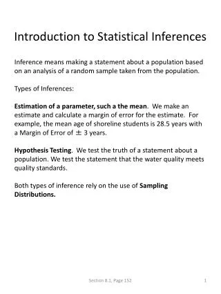
Introduction to Statistical Inferences. Inference means making a statement about a population based on an analysis of a random sample taken from the population. Types of Inferences:

Introduction to Statistical Inferences
E N D
Presentation Transcript
Introduction to Statistical Inferences Inference means making a statement about a population based on an analysis of a random sample taken from the population. Types of Inferences: Estimation of a parameter, such a the mean. We make an estimate and calculate a margin of error for the estimate. For example, the mean age of shoreline students is 28.5 years with a Margin of Error of ± 3 years. Hypothesis Testing. We test the truth of a statement about a population. We test the statement that the water quality meets quality standards. Both types of inference rely on the use of Sampling Distributions. Section 8.1, Page 152
Confidence Interval for Mean, μwith known σ A random sample of 36 rivets is selected and each is tested for shearing strength. The sample mean = 924 lbs, σ = 18. Our point estimate for the mean shearing strength for the entire population would beμ =924 lbs. Because this is just one sample, it is unlikely that the sample mean of 924 lbs. exactly equals the true mean of the population. How close is the sample mean to the true mean of the population? We will use the sample mean to develop and confidence interval or range of numbers for the plausible value of the true mean. Section 8.1, Page 154
Confidence Interval for Mean, μwith known σ Because the sampling is normal, we know that the area between μ – 6 and μ+6 contains 95% of all the sample means. If I pick a sample mean at random and construct an interval ( -6, +6), there is a 95% chance that this will be within 6 units of the true mean, and the interval will therefore contain the true mean. For our example, = 924, our 95% confidence interval is (918, 930) Section 8.1, Page 154
Confidence Interval for Mean, μwith known σ When a sampling distribution for a sample mean, is normal, then a confidence interval for μ, the true mean as follows: Confidence Interval = ± Margin of Error Margin of Error = Critical Value × Standard Error. The critical value sometimes referred to as confidence coefficient is the number of standard error units in the Margin of Error for a given confidence level. We will use the notation z(α) to refer to to the critical value for the confidence level α. The equation for the confidence interval for confidence α: ± Margin of Error = ± z(α) × Section 8.2, Page 156
Constructing An IntervalTI-83 Add-in Programs A random sample of 100 commuting students was obtained. The resulting sample mean was 10.22 miles. (σ = 6 miles) Find the 95% confidence interval for the true mean. Check conditions: Since the sample size is ≥ 30, the sampling distribution will be normal, even if the population is not normal. C. I. = sample mean ± margin of error = sample mean ± critical value * standard error. Find the critical value for 95% confidence. PRGM – 1:CRITVAL – ENTER 1 ENTER - .95 - ANSWER: CR VALUE = 1.96 Find the Standard Error of the Sampling Distribution PRGM – STDERROR-ENTER 4:1 MEAN : 100 : 6 : ANSWER: SE = .60 C.I. = 10.22 ± 1.96 * 0.60 = 10.22 ± 1.176C.I. = (10.22 – 1.176, 10.22 + 1.176 = (9.04, 11.40) Section 8.2, Page 157
Constructing An IntervalBlack Box Program • A random sample of 100 commuting students was obtained. The resulting sample mean was 10.22 miles. (σ = 6 miles) Find the 95% confidence interval for the true mean. • STAT - TESTS – 7:Zinterval – ENTER • STATS : σ = 6 ; = 10.22 ; n=100 ; C-Level = .95 • Answer: (9.04, 11.40) • Using this output we can say: • We are 95% confident that the true mean commute distance is in the the interval. • If we were to take 100 different samples, and construct 100 different confidence intervals, approximately 95 of them would contain the true mean commute distance. • Find the Margin of Error for the confidence interval. • ME = .5(width of interval) = .5( 11.40 - 9.04) = 1.18. Section 8.2, Page 157
Problems Problems, Page 50
Problems • What is the variable being studied? • Find the 90% confidence interval estimate for the mean speed. • Find the 95% confidence interval estimate for the mean speed. • Which interval is larger. Why? Problems, Page 178
Sample SizeTI-83 Add-in Program To solve this problem, we need a relationship between sample size and the variables given. The margin of error (ME) is such a relationship. We solve using the TI-83: PGRM – SAMPLSIZ – ENTER – 3: KNOWN σx ; CONF LEVEL = .99; ME = 75; σx = 900; Answer: n = 956 Section 8.2, Page 160
Problems the standard deviation is 5 seconds. Problems, Page 179
Hypothesis Testing The evidence for Ha is the sample mean Ho: The average GPA of students who take statistics is 3.30 (or more) Ha: The average GPA of students who take statistics is less than 3.30. Sample evidence in the form of the sample mean of a sample of students will try to prove Ha is true. If Ha is true, then Ho is false. Section 8.3, Page 161
Writing Hypotheses State authorities suspect the the manager of investment fund is guilty of embezzling money for his own use. In our system of justice, a presumption of innocence is essential to a trial procedure. Ho: Manager is innocentHa: Manager is not innocent The state will present evidence in trial to try to prove Ha. Section 8.3, Page 162
Problems Problems, Page 179
Problems Problems, Page 179
Hypothesis Test of Mean μ (σ Known)Illustrative Problem • Problem: An aircraft manufacturer must demonstrate that its rivets meet the required specifications. One of the specs is: “The mean shearing strength of all such rivets, μ, is at least 925 lbs. (σ=18). Each time the manufacturer buys rivets, it is concerned that the mean strength might be less than the 925-lb pound specification. A random sample of 50 rivets is selected. The sample mean is 921.18 and n = 50. • STEP 1: The set up • a. Describe the parameter of interest. • The parameter of interest is μ, the population mean. • Write the Hypotheses. • Ho: μ = 925 (≥) (The mean is at least 925) • Ha: μ < 925 (The mean is less than 925) Section 8.4, Page 167
Illustrative Problem (2) • STEP 2: Check assumptions for Normal Sampling Distribution • Since σ is known, we will need a normal sampling distribution. The sampling will be normal if the population is normal, or if the sample size is ≥ 30. Since the sample size is 50, the Central Limit Theorem insures that that the sampling distribution is normal • STEP 3: The evidence for Ha • The evidence for Ha is that the sample mean is 921.18 lbs. This is less than the Ho value of 925 lbs. The are two possible explanations for the difference between the sample mean and the Ho mean: • Samples are subject to sampling variation. Ho is true and the sample mean difference is explained by natural sampling variation. • The difference is too great to be reasonably explained by sampling variation. The difference is explained by the fact that Ho is not true. Section 8.4, PLage 169
Illustrative Problem (3) STEP 4. The probability distribution. We will use the probability distribution to calculate the probability that if Ho, is true, the difference between the evidence, and is due to sampling variation. p-value = area =0.0667. Sampling Distribution PRGM – NORMDIST -1 LOWER BOUND = -2ND EE 99 UPPER BOUND = 921.18 MEAN = 925 ANSWER: AREA = p-value = 0.0667. Section 8.4, Page 169
Illustrative Problem (4)Using Black Box Program to Calculate p-value Problem: An aircraft manufacturer must demonstrate that its rivets meet the required specifications. One of the specs is: “The mean shearing strength of all such rivets, μ, is at least 925 lbs (σ=18) . Each time the manufacturer buys rivets, it is concerned that the mean strength might be less than the 925-lb pound specification. A random sample of 50 rivets is selected. The sample mean is 921.18 and n = 50. STAT-TESTS-1:Ztest Input: Stats μo: 925 (This is the Ho parameter value, μ=925) σ: 18 : 921.18 n: 50 μ: <μ0 (The is the alternate Hypotheses) Calculate Answer: P =0.0667 = p-value Section 8.4, Page 169
Illustrative Problem (5) • STEP 5. Decision • We only have two choices for a decision: • We reject Ho • We fail to reject Ho • Recall that there were only two possibilities that could explain the difference between the Ho mean and the sample mean: • Ho is true and the difference is due to sampling variation. • Ho is not true. • The p-value tells us how likely it is that a. is the correct explanation for the evidence. If a. is unlikely – it has a very small probability of occurring- then we conclude b. must be the correct explanation for the evidence, the sample mean. • Decision Criteria (Significance Level for p-value) • If the p-value falls below the significance level, α, then a. is considered too unlikely, and we reject Ho, and conclude Ha is true. If α is not specifically stated in the problem, it is assumed to be 0.05. • Since our problem has a p-value of 0.0667 > 0.05, we fail to reject Ho. Section 8.4, Page 177
What does the P-value really mean? The p-value is a probability! It is the probability that, if H0 is true, the difference between the H0 value and the sample statistic is due to sampling variation. If the p-value is very small, then the difference between the H0 value and the sample statistic is unlikely due to sampling variation, so we must conclude that sampling variation is an unlikely explanation for the difference. We therefore conclude that HA must be true. Sometimes, in the press, we see that a study was inclusive because the study results are likely caused by chance. Or, that the study results are conclusive because the results are unlikely due to chance. In this case, “chance” means normal sampling variation. We also say that the results of the study are not “statistically significant.” There is nothing really “statistically significant” when the null hypothesis is not proved. On the other hand, when null hypothesis is proved, it is a “big deal” and we say the results are “statistically significant.” Section 8.4
Problems • Write the appropriate hypotheses. • What condition must be met? Is it met? Explain. • What is its mean and standard error of the sampling distribution? • Find the p-value. • What is your decision? Explain. Problems, Page 180
Problems • Write the appropriate hypotheses. • What condition must be met? Is it met? Explain. • Sketch the sampling distribution and show its mean and standard deviation? • Find the p-value. • What is your decision? Explain. Problems, Page 181
Two Tailed Test In this problem, sample evidence larger than the mean or evidence smaller than the mean can cause us to reject the null hypothesis. The appropriate hypotheses are: Ho: μ = 82 (The new test mean test value is 82) Ha: μ ≠ 82 (The new test mean is either larger than 82 or smaller than 82) Section 8.4, Page 171
Two Tailed Test Continued P-value = sum of the two symmetrical areas μ=82 Left Tail: PRGM - NORMDIST 1 LOWER BOUND = -2ND EE99 UPPER BOUND = 79 MEAN = 82 ANSWER: 0.0122 p-value = Left tail area + right tail area = 2*Left tail area =0.0244. Since the p-value is less than 0.05, we reject the null hypothesis and conclude the alternative hypothesis is true – the mean of the new test is different than the mean of the old test. Section 8.4, Page 171
Problems • Test the claim that the BMI of the cardiovascular technologists is different than the BMI of the general population. Use α = .05. Assume the population of the BMI of the cardiovascular technologists is normal. • State the necessary hypotheses. • Is the sampling distribution normal. Why? • Find the p-value. • State your conclusion. • If you made an error, what type of error did you make? Problems Page 181
Types of Errors Type I Error: Reject a true H0.Type II Error: Failure to reject a false H0. The probability of a Type I error is the α level or significance level. Recall that we reject Ho if the p-value is 5% or less. If the p-value =5%, there is a 5% chance that the scenario of Ho true and the evidence is due to sampling variation is the correct scenario. In the long run, we will make an error rejecting Ho 5% of the time. We can reduce the probability of a type I error by reducing the α level to 1%. If the p-value =1%, there is a 1% chance that the scenario of Ho true and the evidence is due to sampling variation is the correct scenario. In the long run, we will make a type I error only 1% of the time. Reducing the α level will reduce the probability of a type I error, but it will increase the probability of a type II error, fail to reject a false Ho. Section 8.3, Page 162
Problems Problems, Page 179
Problems Problems, Page 179