Understanding Slope Fields and Euler's Method for Differential Equations
This guide delves into the fundamentals of differential equations, focusing on slope fields and Euler’s Method. You'll learn how differential equations involve derivatives and how the order is determined by the highest derivative present. We'll explore first-order differential equations and initial-value problems, illustrating how to find unique solutions given initial conditions. The construction of slope fields through approximation will be demonstrated, showcasing how to visualize differential equation solutions. Additionally, Euler’s Method will be explained as a powerful tool for graphing these solutions.

Understanding Slope Fields and Euler's Method for Differential Equations
E N D
Presentation Transcript
6.1 Slope Fields and Euler’s Method
What you’ll learn about • Differential Equations • Slope Fields • Euler’s Method … and why Differential equations have been a prime motivation for the study of calculus and remain so to this day.
Differential Equation An equation involving a derivative is called a differential equation. The order of a differential equation is the order of the highest derivative involved in the equation.
First-order Differential Equation If the general solution to a first-order differential equation is continuous, the only additional information needed to find a unique solution is the value of the function at a single point, called an initial condition. A differential equation with an initial condition is called an initial-value problem. It has a unique solution, called the particular solution to the differential equation.
Example Using the Fundamental Theorem to Solve an Initial Value Problem
Slope Field The differential equation gives the slope at any point (x, y). This information can be used to draw a small piece of the linearization at that point, which approximates the solution curve that passes through that point. Repeating that process at many points yields an approximation called a slope field.
1. Begin at the point ( , ) specified by t x y he initial condition. 2. Use the differential equation to find the slope / at the point. dy dx 3. Increase by . Increase by , where x x y y D D y dy dx x (x + Dx, y + Dy) D = D ( / ) . This defines a new point that lies along the linearization. 4. Using this new point, return to step 2. Repeating the process constructs the graph to the righ t of the initial point. 5. To construct the graph moving to the left from the initial point,repeat the process using negative values for . x D Euler’s Method for Graphing a Solution to an Initial Value Problem