Download

1 / 26
270 likes | 600 Vues
A Three Dimensional Lotka-Volterra System. Kliah Soto Jorge Munoz Francisco Hernandez. Two-Dimensional Case. Extreme Cases. and . Equilibria. Solution Curves. Solve the system of equations:. Solution Curve. Pink: prey x Blue: predator y. Solution curve with all parameters = 1.

E N D
A Three Dimensional Lotka-Volterra System Kliah Soto Jorge Munoz Francisco Hernandez
Extreme Cases and
Solution Curves Solve the system of equations:
Solution Curve Pink: prey x Blue: predator y Solution curve with all parameters = 1
Extremities Case 1: if z=0 then we have the 2 dimensional case Case 2: y=0
In the absence of the middle predator y, we are left with: We combine it to one fraction and use separation of variables: species z approaches zero as t goes to infinity, and species x exponentially grows as t approaches infinity.
Phase Portrait and Solution Curve when y=0 The blue curve represents the prey, while the red curve represents the predator.
In the absence of the prey x, we are left with: We combine it to one fraction and use separation of variables: species y and z will approach zero as t approaches infinity.
Phase Portrait and Solution Curve when x=0 The blue curve represents the top predator, while the red curve represents the middle predator.
Equilibria Set all three equations equal to zero to determine the equilibria of the system:
Cases of Equilibria x=0 and y=0 since a and f are positive. Again equilibrium (0,0,0). When x=0: Either y=0 or z=-c/e z has to be positive so we conclude that y=0 making the last equation z=0. Equilibrium at (0,0,0) When y=0 System reduces to:
Either z= 0 or –f+gy =0. Taking the first case will result in the trivial solution again as well as the equilibrium from the two dimensional case. (c/d,a/b,0) Using parameterization we set x=s and the last equilibrium is: Equilibrium point at (s,a/b=f/g,(ds-c)/e) When we consider:
Linearize the System by finding the Jacobian Where the partial derivatives are evaluated at the equilibrium point
Center Manifold Theorem Real part of the eigenvalues Positive: Unstable Negative: Stable Zero: Center Number of eigenvalues: Dimension of the manifold Manifold is tangent to the eigenspace spanned by the eigenvectors of their corresponding eigenvalues
Equilibrium at (0,0,0) One-dimensional unstable manifold: curve x-axis Two-dimensional stable manifold: surface yz- Plane • Eigenvalues: • a, -c, -f • Eigenvectors: • {1,0,0}, {0,1,0}, {0,0,1}
Solution: • Unstable x-axis • Stable yz-Plane
Equilibrium at (c/d, a/b, 0) Eigenvalues Eigenvectors:
One-Dimensional invariant curve: Stable if ga<fb Unstable ga>fb Two-Dimensional center manifold Three-dimensional center manifold If ga=fb
Stable Equilibrium ga<fb Blue represents the prey. Pink is the middle predator Yellow is the top predator (2,2,2) All parameters equal 1 a = 0.8
Unstable Equilibrium ga>fb Blue represents the prey. Yellow is the middle predator Pink is the top predator (2,2,2) a=1.2 , b=c=d=e=f=g=1
Three Dimensional Manifold ga=fb All parameters 1 initial condition (1,2,4) Blue represents the prey. Pink is the middle predator Yellow is the top predator
Conclusion The only parameters that have an effect on the top predator are a, g, f and b. Large values of a and g are beneficial while large values of f and b represent extinction. The parameters that affect the middle predator are c, d and e. They do not affect the survival of z. The survival of the middle predator is guaranteed as long as the prey is present. The top predator is the only one tha faces extinction when all species are present. Eigenvalues for (c/d, a/b,0)