Download
1 / 26
260 likes | 285 Vues
Clustering Microarray Data based on Density and Shared Nearest Neighbor Measure. CATA’06, March 23-25, 2006 Seattle, WA, USA Ranapratap Syamala, Taufik Abidin, and William Perrizo Dept. of Computer Science North Dakota State University Fargo, ND, USA. Outline. Microarrays Significance

E N D
Clustering Microarray Data based on Density and Shared Nearest Neighbor Measure CATA’06, March 23-25, 2006 Seattle, WA, USA Ranapratap Syamala, Taufik Abidin, and William Perrizo Dept. of Computer Science North Dakota State University Fargo, ND, USA North Dakota State University
Outline • Microarrays • Significance • Objectives of Microarray Data Analysis • Related works • The proposed clustering algorithm • Definitions • The clustering algorithm • Results • Conclusion and Future work North Dakota State University
Microarrays: significance • One of the biggest breakthroughs in the field of genomics for monitoring genes (high throughput technology) • Useful in studying patterns of co-expression in genes • Co-expressed genes: • Genes that exhibit similar expression profiles • over time (or over an experiment series or both) • Useful in identifying functional categories of a group of genes, how genes interact to form interaction networks, etc. • Coherent pattern: A common trend exhibited by the co-expressed genes North Dakota State University
Objectives of Microarray Data Analysis • Large amounts of data are being generated • Our Objectives: • Class discovery: The goal is to identify the clusters of genes that have similar gene expression profiles over a time series of experiments. • Clustering is the main technique employed in class discovery. • Class prediction:Assigning an unclassified gene to a class using similarity of expression pattern with the genes in a particular class. • Classification is the main technique used in class prediction. • Class comparison:Aims at identifying and describing the differences in expression profiles between classes. • identifying a "typical" or "canonical" element or something that differentiates the elements of different classes.
Class Discovery/Clustering • In microarray data analysis, genes exhibiting similar gene expression profiles are considered to be similar (in terms of the graph shape, not the magnitude). • common expression patterns are clustered together. • Pearson’s Correlation Coefficient (PCC)is commonly used to assess this kind of similarity of genes. (x,y) = cov(x,y) / x x • A similarity matrix is constructed consisting of the PCC coefficients between pairs of genes. • The higher the coefficient, the greater the similarity North Dakota State University
Related work • Partition-based clustering: Given a database of n objects and k clusters, the objects are organized into k disjoint partitions, each partition representing a cluster • K-means and K-medoids Clustering • Hierarchical clustering: Agglomerative and Divisive based on the construction of hierarchy • AGNES, DIANA • Density-based clustering: Discovers clusters of arbitrary shapes and effectively filters out noise based on the notion of density and connectivity • DBSCAN, OPTICS, DENCLUE North Dakota State University
Limitations • Partition-based clustering methods: • Must choose the number of clusters, k, before you know anything about them (a priori). • Almost always produce spherical (isotropic) clusters. • Hierarchical clustering methods: • Highly depend on the execution of the merge or split decision of the branches and is greedy (no backtracking), thus can lead to low quality clusters. • Does not scale well to large data sets. • Density (Connectivity) -based clustering methods • Do not scale well to large data sets. North Dakota State University
The Proposed Clustering Algorithm • Addresses the problem of • a priori knowledge of clusters (needing to know k). • produces clusters of arbitrary shape. • improved scaling to large data sets. • Based on the notions of • density • shared nearest neighbors. • P-tree1 technology for scalable data mining 1P-tree technology is patented by NDSU. United States Patent No. 6,941,303. North Dakota State University
R[A1] R[A2] R[A3] R[A4] 2 7 6 1 6 7 6 0 2 7 5 1 2 7 5 7 5 2 1 4 2 2 1 5 7 0 1 4 7 0 1 4 010 111 110 001 011 111 110 000 010 110 101 001 010 111 101 111 101 010 001 100 010 010 001 101 111 000 001 100 111 000 001 100 010 111 110 001 011 111 110 000 010 110 101 001 010 111 101 111 101 010 001 100 010 010 001 101 111 000 001 100 111 000 001 100 = R11 R12 R13 R21 R22 R23 R31 R32 R33 R41 R42 R43 0 1 0 1 1 1 1 1 0 0 0 1 0 1 1 1 1 1 1 1 0 0 0 0 0 1 0 1 1 0 1 0 1 0 0 1 0 1 0 1 1 1 1 0 1 1 1 1 1 0 1 0 1 0 0 0 1 1 0 0 0 1 0 0 1 0 0 0 1 1 0 1 1 1 1 0 0 0 0 0 1 1 0 0 1 1 1 0 0 0 0 0 1 1 0 0 0 0 0 1 0 01 0 1 0 1 0 0 1 0 0 1 01 P11 P12 P13 P21 P22 P23 P31 P32 P33 P41 P42 P43 0 0 0 0 1 01 0 0 0 0 1 0 0 10 01 0 0 0 1 0 0 0 0 0 0 0 1 01 10 0 0 0 0 1 10 0 1 0 ^ ^ ^ ^ ^ ^ ^ ^ ^ 0 0 1 0 1 0 0 1 0 1 01 0 1 0 P-tree overview R(A1 A2 A3 A4) Predicate tree technology: vertically project each attribute vertically project each bit position of each attribute, compress each bit slice into P-tree Basic logical operations performed horizontally across these P-trees (rather than massive vertical scans) North Dakota State University
Definitions • NN(g) = {gj | sim(g,gj) threshold }. • density (g) =gjNN(g)sim(g,gj) • PNN(g) is a P-tree mask for NN(g) ( i.e., the predicate is gjNN(g) ) • shared nearest neighbors measure: snn(gi,gj)= size( NN(gi) ∩ NN(gj) ) • snn determination is scalable (one P-tree AND operation): snn (gi, gj) = rootCount ( PNN(gi) PNN(gj) ) North Dakota State University
Definitions • Core gene: A gene, g, with highest density in its near neighborhood set, NN(g) • Border gene: If NN( g) contains at least one gene with higher density than g(and that nbr gene is not core), then g is called a border gene • Noise: If |NN(gi)| is zero, we consider that gene as noise (in a cluster all by itself). North Dakota State University
The Clustering Algorithm • Identify the two genes with highest density from the as yet unprocessed genes. • Find the nearest neighbor sets of both the genes • if # shared nbrs > snnThreshold (e.g.,2) • then process all these points into the same cluster (creating a new cluster) with the highest density core gene designated its identifier. North Dakota State University
The Clustering Algorithm contd… • If the two genes do not share enough neighbors, then process each gene separately as follows • If it is a core gene, then process it and its neighbors into a cluster, • else (not a core gene) designate it a border gene (note: can't happen in the 1st round) • At any point, a noise gene can can be identified (no near neighbors) and be so designated. • Continue until all genes are processed. North Dakota State University
Procedure: Clustering based on density and shared nearest neighbors Input: All genes and noise true/false Output: Clusters of genes BEGIN: WHILE (unprocessedgenes > 0) DO mostDenseGenes findTwoMostDensegenes, (gi,gj) (unprocessedGenes) processedGenes.add mostDenseGenes getNeighbors (mostDensegenes, simThreshold) IF noNeighbors (mostDensegenes) THEN noisegenes.add mostDensegenes ELSE IF rootCount (NNm (gi) NNm (gj)) > snnThreshold THEN clusterNeighbors() (NN(gi) NN(gj)) processedgenes.add neighbors(mostDensegenes) ELSE FOR i=1 TO mostDensegenes.size () DO currentgene mostDensegenes[i] IF currentgene has Neigbors THEN IF isCore (currentGene) THEN coreGenes.add currentGene neighbors processNeighbors (currentgene) clusterNeighbors () ELSE borderGenes.add currentGene END IF ELSE noiseGenes.add currentGene END IF END FOR END IF Update unprocessedGenes END WHILE END North Dakota State University
The Clustering Algorithm contd… Assigning the border genes to clusters using vertical P-tree mask anding Case I: The border gene, b, share neighbors with clusters (assign to the cluster with max shared nbrs) PNN(b) PC1 PC2 PC3 PC4 0 1 0 0 1 0 1 0 0 0 1 0 0 1 0 0 0 1 0 0 0 1 1 0 0 0 1 0 0 0 00 0 1 0 0 0 1 0 0 0 0 0 0 1 0 0 0 1 0 1 0 0 0 1 0 0 0 1 0 0 0 1 0 1 0 0 0 1 0 0 0 1 0 0 0 1 0 1 0 0 0 1 0 0 0 1 0 0 0 1 0 1 0 0 0 1 0 0 0 1 0 0 0 1 0 1 0 0 0 1 0 1 0 1 0 0 0 0 0 0 0 0 1 0 0 AND with each of the cluster masks Root count of AND operation 1 1 2 0 Case II: The border gene does not share neighbors with any cluster, then it is assigned to the cluster with the most similar core gene identifier North Dakota State University
109 genes 14 2.5 12 2 10 1.5 8 1 6 0.5 4 0 2 1 2 3 4 5 6 7 8 9 10 11 12 0 1 2 3 4 5 6 7 8 9 10 11 12 SimilarityThreshold =0.90, snn=20, execution time = 5.7 sec Results 103 genes This slide shows the clustering of Iyer’s data set, which contains 517 genes with expression levels measured at 12 time points. We discovered 13 clusters, the top 3 (in terms of size) are shown. We also know which are the border genes and can examine them separately when there is good reason to do so (e.g., see next slide). 70 genes 12 10 8 6 4 2 0 1 2 3 4 5 6 7 8 9 10 11 12
41 genes 90 80 70 60 50 40 30 20 10 0 1 2 3 4 5 6 7 8 9 10 11 12 Results-2 The 4th ranking cluster (in terms of size) has a border gene which expresses quite differently at time point = 6 , somewhat differently for time points = 5,7 and then slightly but significantly differently at time points 8 and 9. That gene should probably be examined individually (using biological domain knowledge) to determine if it should be reclassified.
Conclusion and future work • A new clustering algorithm based on density and shared nearest neighbors is presented. • It automatically determines the number of clusters and identifies clusters of arbitrary shape and size • It scales well due to the use of vertical P-tree technology. • Does no horizontal record scans. • Does AND and OR operations on vertical P-tree structures • Future work: • Explore sub-clustering based on different snnThreshold • Develop the Visualization and an interactive exploration of the results. North Dakota State University
Table 1. Clustering accuracy on Yeast cell cycle data set F S c o r e • The table shows the clustering accuracy (F-Score) by different clustering algorithms on Yeast cell cycle microarray data. As can be seen, our approach out-performs the other algorithms in 3 of the cases and produce comparable results with k-means. • But k-means depend on the input order and generate different results every time. • F-score = • where P=Precision = true_positives/(true_positives+false_positives) • R= recall = true_positives/|N|, N=no. of genes in the original cluster North Dakota State University
Table 2. Effect of Similarity threshold The table shows the number of clusters generated by different clustering algorithms on Iyer’s data. As can be seen, our approach provides the number of clusters close to the number of clusters previously reported (10 clusters) in the literature. North Dakota State University
The algorithms that have been used for performance analysis were web-based applications and have been referred in different research papers. The UNIX compatible code is not available for scalability/speed comparisons. The main focus of our performance was on the accuracy of different algorithms (Table 1), and how the clustering algorithms perform with different similarity threshold (input parameter for all the algs), which is also an important parameter for the biologist when they perform comparative analysis of genes and understand their behavior among different species. North Dakota State University
Pearson's correlation coefficient exampleA commonly used formula is X Y 1 2 2 5 3 6 scalar product L1 or Manhattan vector length squared-L2 (Euclidean) vector length Note: Change Y to 2,4,6 (colinear with X but twice as long): 28 - 24 4 r = ------------------------------ = ------------ = 1 SQRT((14-12)(56-48)) SQRT(16) So what are we measuring here? Angle between vectors? Why not just use Arcos(xoy/|x||y|)? Or just cos of the angle between them which is xoy / (|X| |y|)? Vector Space dimension
Pearson's correlation coefficient examplez-score formula A simpler looking formula can be used if the numbers are converted into z scores, where zx is the variable X converted into z scores and zy is the variable Y converted into z scores. The standard normal distribution is a normal distribution with a mean of 0 and a standard deviation of 1. Normal distributions can be transformed to standard normal distributions by the formula:where X is a score from the original normal distribution, μ is the mean of the original normal distribution, and σ is the standard deviation of original normal distribution. The standard normal distribution is called the z distribution. A z score always reflects the number of standard deviations above or below the mean a particular score is. For instance, if a person scored a 70 on a test with a mean of 50 and a standard deviation of 10, then they scored 2 standard deviations above the mean. Converting the test scores to z scores, an X of 70 would be:So, a z score of 2 means the original score was 2 standard deviations above the mean. Note that the z distribution will only be a normal distribution if the original distribution (X) is normal. North Dakota State University
Pearson's correlation coefficient examples North Dakota State University
Appendix (wikipedia on Pearson's Coef.) Pearson's product-moment coefficient Mathematical properties The correlation ρX, Y between two random variables X and Y with expected values μX and μY and standard deviations σX and σY is defined as: Since μX = E(X), σX2 = E(X2) − E2(X) and likewise for Y, also write: The correlation is defined only if both standard deviations are finite and both of them are nonzero. It is a corollary of the Cauchy-Schwarz inequality that the correlation cannot exceed 1 in absolute value. The correlation is 1 in the case of an increasing linear relationship, −1 in the case of a decreasing linear relationship, and some value in between in all other cases, indicating the degree of linear dependence between the variables. The closer the coefficient is to either −1 or 1, the stronger the correlation between the variables. If the variables are independent then the correlation is 0, but the converse is not true because the correlation coefficient detects only linear dependencies between two variables. Here is an example: Suppose the random variable X is uniformly distributed on the interval from −1 to 1, and Y = X2. Then Y is completely determined by X, so that X and Y are dependent, but their correlation is zero; they are uncorrelated. However, in the special case when X and Y are jointly normal, independence is equivalent to uncorrelatedness. A correlation between two variables is diluted in the presence of measurement error around estimators of one or both variables, in which case disattenuation provides a more accurate coefficient. The sample correlation: If we have a series of n measurements of X and Y written as xi and yi where i = 1, 2, ..., n, then the Pearson product-moment correlation coefficient can be used to estimate the correlation of X and Y . The Pearson coefficient is also known as the "sample correlation coefficient". It is especially important if X and Y are both normally distributed. The Pearson correlation coefficient is then the best estimate of the correlation of X and Y . The Pearson correlation coefficient is written: where and are the sample means of xi and yi , sx and sy are the sample standard deviations of xi and yi and the sum is from i = 1 to n. As with the population correlation, we may rewrite this as Again, as is true with the population correlation, the absolute value of the sample correlation must be less than or equal to 1. Though the above formula conveniently suggests a single-pass algorithm for calculating sample correlations, it is notorious for its numerical instability (see below for something more accurate).
Appendix (wikipedia on Pearson's Coef.) -2 The sample correlation coefficient is the fraction of the variance in yi that is accounted for by a linear fit of xi to yi . This is written where σy|x2 is the square of the error of a linear fit of yi to xi by the equation y = a + bx and σy2 is just the variance of y Note that since the sample correlation coefficient is symmetric in xi and yi , we will get the same value for a fit of xi to yi : This equation also gives an intuitive idea of the correlation coefficient for higher dimensions. Just as the above described sample correlation coefficient is the fraction of variance accounted for by the fit of a 1-dimensional linear submanifold to a set of 2-dimensional vectors (xi , yi ), so we can define a correlation coefficient for a fit of an m-dimensional linear submanifold to a set of n-dimensional vectors. For example, if we fit a plane z = a + bx + cy to a set of data (xi , yi , zi ) then the correlation coefficient of z to x and y is Non-parametric correlation coefficients: Pearson's correlation coefficient is a parametric statistic, and it may be less useful if the underlying assumption of normality is violated. Non-parametric correlation methods, such as Spearman's ρ and Kendall's τ may be useful when distributions are not normal; they are a little less powerful than parametric methods if the assumptions underlying the latter are met, but are less likely to give distorted results when the assumptions fail. Other measures of dependence among random variables: To get a measure for more general dependencies in the data (also nonlinear) it is better to use the correlation ratio which is able to detect almost any functional dependency, or mutual information which detects even more general dependencies. Copulas and correlation: Most people erroneously believe the info given by a correlation coef. is enough to define the dependence structure between random variables. But to fully capture the dependence between random variables we must consider the copula between them. The correlation coefficient completely defines the dependence structure only in particular cases, for example when the cumulative distribution functions are elliptic (as with, for example, the multivariate normal dist). Correlation matrices: The correlation matrix of n random variables X1, ..., Xn is the n × n matrix whose i,j entry is corr(Xi, Xj). If the measures of correlation used are product-moment coefficients, the correlation matrix is the same as the covariance matrix of the standardized random variables Xi /SD(Xi) for i = 1, ..., n. Consequently it is necessarily a non-negative definite matrix. The correlation matrix is symmetrical (correlation between Xi and Xj is the same as the correlation between Xj and Xi). Correlation does not imply causation: The conventional dictum that "correlation does not imply causation" is treated in the article titled spurious relationship. See also correlation implies causation (logical fallacy). However, correlations are not presumed to be acausal, though the causes may not be known. Computing correlation accurately in a single pass: The following algorithm (in pseudocode) will estimate correlation with good numerical stability: sum_sq_x = 0 sum_sq_y = 0 sum_coproduct = 0 mean_x = x[1] mean_y = y[1] last_x = x[1] last_y = y[1] for i in 2 to N: sweep = (i - 1.0) / i delta_x = x[i] - mean_x delta_y = y[i] - mean_y sum_sq_x += delta_x * delta_x * sweep sum_sq_y += delta_y * delta_y * sweep sum_coproduct += delta_x * delta_y * sweep mean_x += delta_x / i mean_y += delta_y / i pop_sd_x = sqrt( sum_sq_x / N ) pop_sd_y = sqrt( sum_sq_y / N ) cov_x_y = sum_coproduct / N correlation = cov_x_y / (pop_sd_x * pop_sd_y) For an enlightening experiment, check the correlation of {900,000,000 + i for i=1...100} with {900,000,000 - i for i=1...100}, perhaps with a few values modified. Poor algorithms will fail.