Download

1 / 36
360 likes | 621 Vues
Automatic detection and location of microseismic events . Tomas Fischer. Outline. Why automatic How automatic Errors West Bohemia swarm 2000 Hydraulic stimulation in gas field in Texas. Why automatic processing?. Huge datasets Improve productivity Improve data homogeneity

E N D
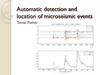
Automatic detection and location of microseismic events Tomas Fischer
Outline • Why automatic • How automatic • Errors • West Bohemia swarm 2000 • Hydraulic stimulation in gas field in Texas
Why automatic processing? • Huge datasets • Improve productivity • Improve data homogeneity • Real time processing – alarms
Utilization of automatic processing • Measurement of arrival times • Measurement of amplitudes • Phase-waveform extraction • Hypocentre location • Source parameters, focal mechanisms • Seismic tomography • Attenuation studies • …
Approaches • Classical - stepwise:(single station / network)1. Phase detection & picking2. Hypocentre location • Simultaneous (seismic network)– source scanning / back-propagation(Kao & Shan, 2003; Drew 2005)
Classical approach – steps • Phase detection – increased signal energy, single station • Phase association – consistency betw. stations • Phase picking – identify phase onset • Location of hypocenters
Phase detection • Transform 3C seismogram to a scalar > 0, characteristic function CF (Allen, 1978) • Find maxima of CF S-wave energy detector ENZl– maximum eigenvalue of signal covariance matrix in a running window
Distinguishing P and S-waves Hierarchic approach • First find S-waves (higher amplitude, horiz. polarization) • Then find P-waves (perpendicular polarization)
Distinguishing P and S-waves Equal approach • evaluate horiz. & vert. polarization • find consecutive intervals of perpendicular polarization (ampl. ratio or hor/vert gives hint to which one is P and S)
Phase association • Simple kinematic (geometric) criteriae.g. t2 < t1+t12 • A-priori information on source position- plane wave consistency • Preliminary location- test the phase consistency by location residual 1 2 Source
Phase picking Find onset – abrupt amplitude increase • STA/LTA(non-overlapping) • Higher statistic momentsKurtosis • Waveform cross-correlation Horiz. Polarization STA/LTA Kurtosis
Automatic location • No special needs (each location algorithm is automatic) • Hydrocarbon reservoir stimulations – linear array of receivers – besides arrival times also backazimuth (polarization) needed => modify the location algorithm to include also the fit to the polarization data
Event location • 2D array (Earth surface) – P-waves sufficient (S-waves beneficial) t3-t4 1 2 t2-t3 3 4 t1-t2
Event location • 1D array (borehole)both P and S-waves needed 1 Map view depth Depth view 1 2 3 4 5 t1>t2>t3=t4<t5
Goodness • Picking success • Amplitude ratio @ pick • Location residual • Location success • Location residual • Sharpness of foci image ? ! Location residual – results from • Unknown structure • Timing errors • Picking errors (Gaussian & gross) => Residual is not a unique measure of picking success
Location residual calibration (remove gross errors) • Training dataset – if manual processing available • Loc. error: difference between manual and automaticlocations 6 samples
Location residual calibration (remove gross errors) • Dataset to be processed Limit for choice of good locations
Swarm 2000 in West Bohemia • 4 SP stations • 0-20 km epicentral distance • synchronous triggered recording
Swarm 2000 Automatic processing Characteristic function • S: maximum eigenvalue of the covariance matrix in horizontal plane (Magotra et al., 1987) • P: sum of the Z-comp. and its derivative (Allen, 1978) Method • S-waves, minimum interval>maximum expected tS-tP • P-waves in a fixed time window prior to S • Only complete P and S pairs processed=> homogeneous dataset
Swarm 2000 in West Bohemia Resulting automatic picks
Swarm 2000 in West Bohemia • >7000 detected events, 4500 well located • Homogeneous catalog downto ML=0.4 • Location error:±100 m horiz. and ±200 m vert.
Automatic locations with RMS<8 smpl.compared with 405 manually located events
1 2 3 4 5 6+7 8 9 Automatic locations of the 2000 swarm P1 a P2
Hydraulic stimulation in gas field 8 3C geophones continuous recording
Hydraulic stimulation in gas field S-wave picker • Get the maximum eigenvalue l(t) of the signal covariance matrix • Find maxima of polarized energy arriving at consistent delays tj to vertical array (derived from expected slowness) • Identify the S-wave onsets tS by STA/LTA detector in a short time window preceding the maxima of L(t) • Measure S-wave backazimuth • Array compatibility check by fitting hodochrone tS(z)byparabola, outliers repicked or removed
Hydraulic stimulation in gas field P-wave picker • Search for signal s polarized in S-ray direction p. We use the characteristic function • Find maxima of P-wave polarized energy Cp(t) arriving at consistent slowness (similar as in S-wave detection) • Identify the P-wave onsets tP by STA/LTA detector in a short time window preceding the maxima of Cp(t) • Measure the P-wave backazimuth • Use Wadati’s relation to remove tP outliers
Fig. 3. Distribution of time differences between automatically and manualy obtained arrival times of test dataset. Hydraulic stimulation in gas field Comparison of manual and auto picks for 296 manually picked events P S
Conclusions • automatic processing useful in case of huge datasets & provides homogeneous results • two approaches • classic – mimics human interpreter • modern – direct search for the hypocentre • classic – network consistency beneficial • two case studies show successful implementation of polarization based picker
Outlines • use waveform cross-correlation for picking