Exploring Parallelism in Computational Science and Engineering Simulations
This presentation covers the classification of simulation applications in Computational Science and Engineering (CSE), focusing on discrete event systems, particle systems, ordinary differential equations (ODEs), and partial differential equations (PDEs). It discusses methods like Euler’s for solving ODEs and highlights the importance of matrix-vector multiplication in parallel computing. Additionally, it addresses graph partitioning techniques for optimizing performance and communication in sparse matrix operations. By understanding these concepts, researchers can enhance simulations across various domains including finance, engineering, and gaming.

Exploring Parallelism in Computational Science and Engineering Simulations
E N D
Presentation Transcript
CS240A: Parallelism in CSE Applications Tao Yang Slides revised from James Demmel and Kathy Yelick www.cs.berkeley.edu/~demmel/cs267_Spr11
Category of CSE Simulation Applications • Discrete event systems • Time and space are discrete • Particle systems • Important special case of lumped systems • Ordinary Differentiation Equations (ODEs) • Location/entities are discrete, time is continuous • Partial Differentiation Equations (PDEs) • Time and space are continuous discrete continuous CS267 Lecture 4
Basic Kinds of CSE Simulation • Discrete event systems: • “Game of Life,” Manufacturing systems, Finance, Circuits, Pacman • Particle systems: • Billiard balls, Galaxies, Atoms, Circuits, Pinball … • Ordinary Differential Equations (ODEs), • Lumped variables depending on continuous parameters • system is “lumped” because we are not computing the voltage/current at every point in space along a wire, just endpoints • Structural mechanics, Chemical kinetics, Circuits, Star Wars: The Force Unleashed • Partial Differential Equations (PDEs) • Continuous variables depending on continuous parameters • Heat, Elasticity, Electrostatics, Finance, Circuits, Medical Image Analysis, Terminator 3: Rise of the Machines • For more on simulation in games, see • www.cs.berkeley.edu/b-cam/Papers/Parker-2009-RTD CS267 Lecture 4
Table of Cotent ODE PDE Discrete Events and Particle Systems
Finite-Difference Method for ODE/PDE Discretize domain of a function For each point in the discretized domain, name it with a variable, setup equations. The unknown values of those points form equations. Then solve these equations
Euler’s method for ODEInitial-Value Problems Straight line approximation y0 x0 h x1 h x2 h x3
Euler Method Approximate: Then: Thus starting from an initial value y0
ODE with boundary value 5 8 http://numericalmethods.eng.usf.edu
Solution Using the approximation of and Gives you http://numericalmethods.eng.usf.edu
Solution Cont Step 1 At node Step 2 At node Step 3 At node http://numericalmethods.eng.usf.edu
Solution Cont Step 4 At node Step 5 At node Step 6 At node http://numericalmethods.eng.usf.edu
Solving system of equations = Graph and “stencil” x x x http://numericalmethods.eng.usf.edu
Compressed Sparse Row (CSR) Format SpMV: y = y + A*x, only store, do arithmetic, on nonzero entries x Representation of A A y Matrix-vector multiply kernel: y(i) y(i) + A(i,j)×x(j) Matrix-vector multiply kernel: y(i) y(i) + A(i,j)×x(j) for each row i for k=ptr[i] to ptr[i+1]-1 do y[i] = y[i] + val[k]*x[ind[k]] Matrix-vector multiply kernel: y(i) y(i) + A(i,j)×x(j) for each row i for k=ptr[i] to ptr[i+1]-1 do y[i] = y[i] + val[k]*x[ind[k]] CS267 Lecture 4
Parallel Sparse Matrix-vector multiplication • y = A*x, where A is a sparse n x n matrix • Questions • which processors store • y[i], x[i], and A[i,j] • which processors compute • y[i] = sum (from 1 to n) A[i,j] * x[j] = (row i of A) * x … a sparse dot product • Partitioning • Partition index set {1,…,n} = N1 N2 … Np. • For all i in Nk, Processor k stores y[i], x[i], and row i of A • For all i in Nk, Processor k computes y[i] = (row i of A) * x • “owner computes”rule: Processor k compute the y[i]s it owns. x P1 P2 P3 P4 y May require communication CS267 Lecture 4
3 2 4 1 5 6 Matrix-processor mapping vs graph partitioning • Relationship between matrix and graph 1 2 3 4 5 6 1 1 11 2 1 1 11 3 1 11 4 11 1 1 5 11 1 1 6 111 1 • A “good” partition of the graph has • equal (weighted) number of nodes in each part (load and storage balance). • minimum number of edges crossing between (minimize communication). • Reorder the rows/columns by putting all nodes in one partition together. CS267 Lecture 7
Matrix Reordering via Graph Partitioning • “Ideal” matrix structure for parallelism: block diagonal • p (number of processors) blocks, can all be computed locally. • If no non-zeros outside these blocks, no communication needed • Can we reorder the rows/columns to get close to this? • Most nonzeros in diagonal blocks, few outside P0 P1 P2 P3 P4 P0 P1 P2 P3 P4 = * CS267 Lecture 4
Graph Partitioning and Sparse Matrices • Relationship between matrix and graph 1 2 3 4 5 6 1 1 1 1 2 1 111 3 1 1 1 4 11 1 1 5 11 1 1 6 11 1 1 3 4 2 1 5 6 • Edges in the graph are nonzero in the matrix: • If divided over 3 procs, there are 14 nonzeros outside the diagonal blocks, which represent the 7 (bidirectional) edges CS267 Lecture 4
Goals of Reordering • Performance goals • balance load (how is load measured?). • Approx equal number of nonzeros (not necessarily rows) • balance storage (how much does each processor store?). • Approx equal number of nonzeros • minimize communication (how much is communicated?). • Minimize nonzeros outside diagonal blocks • Related optimization criterion is to move nonzeros near diagonal • improve register and cache re-use • Group nonzeros in small vertical blocks so source (x) elements loaded into cache or registers may be reused (temporal locality) • Group nonzeros in small horizontal blocks so nearby source (x) elements in the cache may be used (spatial locality) • Other algorithms reorder for other reasons • Reduce # nonzeros in matrix after Gaussian elimination • Improve numerical stability CS267 Lecture 4
Table of Cotent ODE PDE Discrete Events and Particle Systems
Solving PDEs • Finite element method • Finite difference method (our focus) • Converts PDE into matrix equation • Linear system over discrete basis elements • Result is usually a sparse matrix
Class of Linear Second-order PDEs • Linear second-order PDEs are of the form where A - H are functions of x and y only • Elliptic PDEs: B2 - AC < 0 (steady state heat equations) • Parabolic PDEs: B2 - AC = 0 (heat transfer equations) • Hyperbolic PDEs: B2 - AC > 0 (wave equations)
2D Steady State Heat Distribution Ice bath Steam Steam Steam
Solving the Heat Problem with PDE Underlying PDE is the Poisson equation This is an example of an elliptical PDE Will create a 2-D grid Each grid point represents value of state state solution at particular (x, y) location in plate
Finite-difference • Assume f(x,y)=0 • Namely
Matrx vs. graph representation Graph and “5 pointstencil” 4 -1 -1 -1 4 -1 -1 -1 4 -1 -1 4 -1 -1 -1 -1 4 -1 -1 -1 -1 4 -1 -1 4 -1 -1 -1 4 -1 -1 -1 4 -1 -1 4 -1 L = -1 3D case is analogous (7 point stencil) CS267 Lecture 5
Jacobi method for iterative solutions Start with initial values. Iteratively update variables based on equations For i=1 to n for j= 1 to n w[i][j] = (u[i-1][j] + u[i+1][j] + u[i][j-1] + u[i][j+1]) / 4.0; Swap w and u
Gauss Seidel Iterative Method For i = 1, n For j = 1, n u[i][j] = (u[i-1][j] + u[i+1][j] + u[i][j-1] + u[i][j+1]) / 4.0; u
Gauss-Seidel method for equation solving • 2D dependence graph (b) After red/black variable reordering CS267 Lecture 5
Processor Partitioning in Regular meshes Implemented using “ghost” regions. Adds memory overhead • Computing a Stencil on a regular mesh • need to communicate mesh points near boundary to neighboring processors. • Often done with ghost regions • Surface-to-volume ratio keeps communication down, but • Still may be problematic in practice CS267 Lecture 5
Composite mesh from a mechanical structure CS267 Lecture 5
Converting the mesh to a matrix CS267 Lecture 5
Example of Matrix Reordering Application When performing Gaussian Elimination Zeros can be filled Matrix can be reordered to reduce this fill But it’s not the same ordering as for parallelism CS267 Lecture 7
Irregular mesh: NASA Airfoil in 2D (direct solution) CS267 Lecture 5
Irregular mesh and multigrid CS267 Lecture 9
Challenges of Irregular Meshes • How to generate them in the first place • Start from geometric description of object • Triangle, a 2D mesh partitioner by Jonathan Shewchuk • 3D harder! • How to partition them • ParMetis, a parallel graph partitioner • How to design iterative solvers • PETSc, a Portable Extensible Toolkit for Scientific Computing • Prometheus, a multigrid solver for finite element problems on irregular meshes • How to design direct solvers • SuperLU, parallel sparse Gaussian elimination CS267 Lecture 5
Table of Cotent ODE PDE Discrete Events and Particle Systems
Discrete Event Systems • Systems are represented as: • finite set of variables. • the set of all variable values at a given time is called the state. • each variable is updated by computing a transition function depending on the other variables. • System may be: • synchronous: at each discrete timestep evaluate all transition functions; also called a state machine. • asynchronous: transition functions are evaluated only if the inputs change, based on an “event” from another part of the system; also called event driven simulation. • Example: The “game of life:”sharks and fish living in an ocean • breeding, eating, and death • forces in the ocean&between sea creatures CS267 Lecture 4
P4 Repeat compute locally to update local system barrier() exchange state info with neighbors until done simulating P1 P2 P3 P5 P6 P7 P8 P9 Parallelism in Game of Life • The simulation is synchronous • use two copies of the grid (old and new). • the value of each new grid cell depends only on 9 cells (itself plus 8 neighbors) in old grid. • simulation proceeds in timesteps-- each cell is updated at every step. • Easy to parallelize by dividing physical domain: Domain Decomposition • How to pick shapes of domains? CS267 Lecture 4
Regular Meshes (e.g. Game of Life) • Suppose graph is nxn mesh with connection NSEW neighbors • Which partition has less communication? (n=18, p=9) • Minimizing communication on mesh minimizing “surface to volume ratio” of partition 2*n*(p1/2 –1) edge crossings n*(p-1) edge crossings CS267 Lecture 4
Synchronous Circuit Simulation • Circuit is a graph made up of subcircuits connected by wires • Parallel algorithm is timing-driven or synchronous: • Evaluate all components at every timestep (determined by known circuit delay) • Graph partitioning assigns subgraphs to processors • Goal 1 is to evenly distribute subgraphs to nodes (load balance). • Goal 2 is to minimize edge crossings (minimize communication). better edge crossings = 6 edge crossings = 10 CS267 Lecture 4
Asynchronous Simulation • Synchronous simulations may waste time: • Simulates even when the inputs do not change,. • Asynchronous (event-driven) simulations update only when an event arrives from another component: • No global time steps, but individual events contain time stamp. • Example: Game of life in loosely connected ponds (don’t simulate empty ponds). • Example: Circuit simulation with delays (events are gates changing). • Example: Traffic simulation (events are cars changing lanes, etc.). • Asynchronous is more efficient, but harder to parallelize • In MPI, events are naturally implemented as messages, but how do you know when to execute a “receive”? CS267 Lecture 4
Particle Systems • A particle system has • a finite number of particles • moving in space according to Newton’s Laws (i.e. F = ma) • time is continuous • Examples • stars in space with laws of gravity • electron beam in semiconductor manufacturing • atoms in a molecule with electrostatic forces • neutrons in a fission reactor • cars on a freeway with Newton’s laws plus model of driver and engine • balls in a pinball game CS267 Lecture 4
Forces in Particle Systems • Force on each particle can be subdivided force = external_force + nearby_force + far_field_force • External force • ocean current to sharks and fish world • externally imposed electric field in electron beam • Nearby force • sharks attracted to eat nearby fish • balls on a billiard table bounce off of each other • Far-field force • fish attract other fish by gravity-like (1/r^2 ) force • gravity, electrostatics, radiosity in graphics CS267 Lecture 4
Example: Fish in an External Current % fishp = array of initial fish positions (stored as complex numbers) % fishv = array of initial fish velocities (stored as complex numbers) % fishm = array of masses of fish % tfinal = final time for simulation (0 = initial time) dt = .01; t = 0; % loop over time steps while t < tfinal, t = t + dt; fishp = fishp + dt*fishv; accel = current(fishp)./fishm; % current depends on position fishv = fishv + dt*accel; % update time step (small enough to be accurate, but not too small) dt = min(.1*max(abs(fishv))/max(abs(accel)),1); end CS267 Lecture 4
Parallelism in External Forces • These are the simplest • The force on each particle is independent • Called “embarrassingly parallel” • Sometimes called “map reduce” by analogy • Evenly distribute particles on processors • Any distribution works • Locality is not an issue, no communication • For each particle on processor, apply the external force • May need to “reduce” (eg compute maximum) to compute time step, other data CS267 Lecture 4
Parallelism in Nearby Forces • Nearby forces require interaction and therefore communication. • Force may depend on other nearby particles: • Example: collisions. • simplest algorithm is O(n2): look at all pairs to see if they collide. • Usual parallel model is domain decomposition of physical region in which particles are located • O(n/p) particles per processor if evenly distributed. CS267 Lecture 4