Download
1 / 94
940 likes | 957 Vues
Understand the history, methods, and politics of redistricting in the United States while diving into apportionment paradoxes and the impact of court decisions like Baker v. Carr and Reynolds v. Sims.

E N D
The Mathematics of Redistricting Allan Bickle April 8, 2011
The Constitution • The United States Constitution establishes the House of Representatives in Article I, Section II. • “The number of representatives shall not exceed one for every 30,000” people. • George Washington argued that one per 40,000 was inadequate. • “Each state shall have at least one representative.” • Initially, there were 65, allocated specifically in the Constitution.
The Census • “The actual enumeration shall be made within three years after the first meeting of the Congress of the United States, and within every subsequent term of ten years, in such manner as they shall by law direct.” • The 2010 census was completed last year, and local population data has been released. • The official population in 2010 was 308,745,538.
The Number of Representatives • The Constitution does not dictate the number of Representatives (after 1790). • The number was gradually increased until 1911 to keep up with population growth and new states. • After 1911, the number of representatives stayed at 435*. • *Except Briefly when Alaska and Hawaii were added. • Representatives currently represent about 710,000 people on average.
Allocation of Representatives • There are various ways of allocating representatives among the states. • 1790-1830 The “Jefferson method” • 1840 The “Webster method” • 1850-1890 The “Vinton” or “Hamilton” method • 1910, 1930 The method of major fractions • 1940-present The method of equal proportions (Huntington-Hill)
Desirable Properties of Allocations • We would like a method of allocation that satisfies the following properties. • It follows the quota rule: Each of the parties gets one of the two numbers closest to its fair share of seats (if the party's fair share is 7.34 seats, it gets either 7 or 8). • It does not have the Alabama paradox: If the total number of seats is increased, no party's number of seats decreases. • It does not have the population paradox: If party A gets more votes and party B gets fewer votes, no seat will be transferred from A to B.
The Apportionment Paradox • Theorem [Balinski/Young 1982] No apportionment system with at least three districts satisfies these properties. • Alternate forms: • Any apportionment method that does not violate the quota rule must produce paradoxes, and any apportionment method that does not produce paradoxes must violate the Quota Rule. • Provided the number of seats is fixed in advance of the census, all Constitution compliant apportionment methods violate the Quota Rule.
Congressional District Maps • States draw maps dividing the state into districts with one representative per district. • Usually this is done by the state legislature. • Some states use ‘independent’ commissions.
The Politics of District Maps • Drawing congressional districts is an inherently political process. • A particular map may give an advantage to particular politicians or parties, relative to other possible maps. • Such advantages can be more pronounced in oddly shaped districts.
Gerrymandering • An early example of this are the Massachusetts state senate districts passed in 1812. • They were signed into law by Governor Elbridge Gerry, a signer of the Declaration of Independence • One oddly shaped district was compared to a salamander. • Drawing districts for political benefit, often by means of odd shapes, was called Gerrymandering. • A famous political cartoon helped to popularize the concept.
Redistricting • If the number of Congressional districts allocated to a state changes, it must draw new district maps. • During the first half of the 1900s, many states did not draw new districts.
Court Decisions • Baker v. Carr (1962): redistricting is a judicial issue • Reynolds v. Sims (1964): state legislative districts must be roughly equal in population • Westbury v. Sanders (1964): the same for congressional districts • These cases set off the modern decennial redistricting.
Civil Rights Act of 1965 • Wikipedia: “Some judges and proponents of racially drawn congressional districts have interpreted Section 5 of the Act as requiring racial gerrymandering in order to ensure minority representation. The United States Supreme Court in Miller v. Johnson, (1995), overturned a 1992 Congressional redistricting plan which had created minority majority districts in Georgia as unconstitutional gerrymander. In Bush v. Vera, the Supreme Court, in a plurality opinion, rejected Texas's contention that Section 5 required racially-gerrymandered districts.”
Minority-Majority Districts • There has been a push to create more black-majority (later, Hispanic-majority) districts during each redistricting. • Michigan has two black-majority districts based in Detroit.
Redistricting in Michigan • Michigan senate boundaries were frozen 1925-1952 • Following a constitutional convention, Michigan adopted a new constitution in 1963. • In the 1970s and 80s, redistricting was deadlocked and went to the courts. • In the 1970s, the Michigan Supreme Court adopted the democrat plan.
The Apol Standards • In the 1980s, a court appointed Bernie Apol to devise a plan. • He developed what came to be known as the Apol standards. • These were codified into law in 1999. • The 2000 redistricting generally followed these standards. • In the 2001 case LeRoux v. Secretary of State, the Michigan Supreme Court ruled that these standards could not bind future legislatures.
Congressional Redistricting: Standard A • Except as otherwise required by federal law for congressional districts in this state, the redistricting plan shall be enacted using only these guidelines in the following order of priority: • (a) The constitutional guideline is that each congressional district shall achieve precise mathematical equality of population in each district.
Implications of Standard A • Uh Oh! Michigan’s population can’t be divided evenly by 15. • Solution: get as close as possible. • District 10 (Macomb, St. Clair) has one person fewer than all the other districts. • Practically speaking, each district (or proper subset of districts) will ‘break’ at least one county and city/township.
Standard B • (b) The federal statutory guidelines in no order of priority are as follows: • (i) Each congressional district shall be entitled to elect a single member. • (ii) Each congressional district shall not violate section 2 of title I of the voting rights act of 1965, Public Law 89-110, 42 U.S.C. 1973.
Standard C1 • (c) The secondary guidelines in order of priority are as follows: • (i) Each congressional district shall consist of areas of convenient territory contiguous by land. Areas that meet only at points of adjoining corners are not contiguous.
What Does ‘Contiguous’ Mean? • Websters: • in physical contact; touching along all or most of one side • near, next, or adjacent
Connected Spaces • Mathematically, there are various concepts of what it means for a topological space to be connected. • Disconnected: there are disjoint nonempty open sets H and K in X such that X = H U K. • Connected: not disconnected. • Path-connected: for any two points x and y in X, there is a continuous function f mapping the unit interval to X with endpoints x and y. • Path-connectected implies connected, but not conversely. • Example: the topologist’s comb
Cut-points • Cut-point: a point p of a space X so that X-p is disconnected. • Standard C1 seems to imply that districts must be path-connected with no cut-points. • Other states may not use the same definitions. • Example: North Carolina 6 and 13. • Cutting it close with offsets: MI senate 26.
Contiguious By Land • What about the requirement to be contiguous ‘by land’? • Example: 1990s NJ-13 (Albio Sires) • Presumbly, the Mackinaw Bridge counts as land for these purposes.
2-cell Spaces • 2-cell: any closed curve can be continuously contracted to a point in the spacee. • There is no requirement that districts be 2-cell. • Example: 1990s Jackson County state house districts.
Standard C2-5 • (ii) Congressional district lines shall break as few county boundaries as is reasonably possible. • (iii) If it is necessary to break county lines to achieve equality of population between congressional districts as provided in subdivision (a), the number of people necessary to achieve population equality shall be shifted between the 2 districts affected by the shift. • (iv) Congressional district lines shall break as few city and township boundaries as is reasonably possible. • (v) If it is necessary to break city or township lines to achieve equality of population between congressional districts as provided in subdivision (a), the number of people necessary to achieve population equality shall be shifted between the 2 districts affected by the shift.
Analyzing County and City/township Breaks • First, consider city/township breaks. • Recall that there is effectively no chance that any district or proper subset of districts can avoid a break. • For the moment, assume any break splits a city in two/township in two. • How few is ‘reasonably possible’? • Assume we want the minimum possible.
Graphs as Models • A graph is a mathematical object consisting of a set of objects (vertices) and a set of two-element subsets of the vertices (edges). • In this case, we let the vertices represent the districts. • One possibility for the edges is to draw an edge between any pair of districts that share a boundary. • This type of graph is called the dual of a map.
Planar Graphs • A graph is planar if it can be drawn in the plane with no edges crossing. • The graph corresponding to Michigan’s districts is planar. • Is every dual of a congressional district map planar?
A Different Model • In a typical graph theory lecture, I would now start talking about Francis Guthrie… • Instead, we consider a different possibility for the edges. • Draw an edge between vertices if the corresponding districts break (share part of) a city/township. • Call this the break graph for a district map.
Connected Graphs and Cycles • A graph is connected if there is a path (sequence of edges) between any pair of vertices. • The break graph must be connected. • A cycle of a graph is a subgraph whose vertices form a loop. • Given a connected graph, we can successively delete edges from cycles until we obtain a connected graph with no cycles. • A connected graph with no cycles is called a tree.
Trees • The number of edges of a graph is called its size. • To find the minimum number of possible, we want to find the size of a tree. • A leaf of a tree is a vertex that is adjacent to exactly one other vertex. • Lemma. Every tree with at least two vertices has at least two leaves. • Proof. Consider a path of maximum length. If its ends were adjacent more than one vertex, this would create a longer path or a cycle.
Operation Characterization of Trees • Theorem. A graph is a tree if and only if it can be constructed from a single vertex by iterating the operation of adding a new leaf adjacent to one of the existing vertices. • Proof. (→) A single vertex is a tree since it is connected and has no cycles. Adding a new leaf adjacent to an existing vertex preserves both these properties. (←) The theorem is obvious if T is a single vertex. Assume the theorem holds for all trees with fewer than n vertices and let T be a tree with n vertices. By the lemma, T has a leaf v. Then by assumption, T-v can be constructed using the operation. But then adding v back shows that T can as well. Thus the theorem holds by mathematical induction.
The Size of Trees • Corollary. The size of a tree with n vertices is n-1. • Proof. This is certainly true for a single vertex. Every tree can be constructed by successively adding a vertex and an adjacent edge, increasing the number of vertices and the size by one. Thus the result holds for all trees.
Implications • This implies that under our assumptions, the minimum possible number of breaks is one less than the number of districts. • Currently, Michigan has 15 congressional districts and 14 city/township breaks. • Is this always achievable? • Yes. If the break graph contains a cycle, shift population around the cycle to eliminate one of the breaks on the cycle. • No map that minimizes the number of breaks can have two districts that both contain parts of two cities/townships or counties.
Complications • Townships can be disconnected. • Example: Kalamazoo Township is broken into four pieces. • Cities can be surrounded. • Example: Highland Park and Hamtramck are surrounded by Detroit.