CSE 473 Markov Decision Processes
CSE 473 Markov Decision Processes. Dan Weld. Many slides from Chris Bishop, Mausam , Dan Klein, Stuart Russell, Andrew Moore & Luke Zettlemoyer. MDPs. Markov Decision Processes Planning U nder Uncertainty Mathematical Framework Bellman Equations Value Iteration


CSE 473 Markov Decision Processes
E N D
Presentation Transcript
CSE 473 Markov Decision Processes Dan Weld Many slides from Chris Bishop, Mausam, Dan Klein, Stuart Russell, Andrew Moore & Luke Zettlemoyer
MDPs Markov Decision Processes • Planning Under Uncertainty • Mathematical Framework • Bellman Equations • Value Iteration • Real-Time Dynamic Programming • Policy Iteration • Reinforcement Learning Andrey Markov (1856-1922)
Recap: Defining MDPs • Markov decision process: • States S • Start state s0 • Actions A • Transitions P(s’|s, a) aka T(s,a,s’) • Rewards R(s,a,s’) (and discount ) • Compute the optimal policy, * • is a function that chooses an action for each state • We the policy which maximizes sum of discounted rewards
2 4 3 2 High-Low as an MDP • States: • 2, 3, 4, done • Actions: • High, Low • Model: T(s, a, s’): • P(s’=4 | 4, Low) = • P(s’=3 | 4, Low) = • P(s’=2 | 4, Low) = • P(s’=done | 4, Low) = 0 • P(s’=4 | 4, High) = 1/4 • P(s’=3 | 4, High) = 0 • P(s’=2 | 4, High) = 0 • P(s’=done | 4, High) = 3/4 • … • Rewards: R(s, a, s’): • Number shown on s’ if s’<s a=“high” … • 0 otherwise • Start: 3 1/4 1/4 1/2 So, what’s a policy? : {2,3,4,D} {hi,lo}
Bellman Equations for MDPs • <S, A, Pr, R, s0, > • Define V*(s) {optimal value} as the maximum expected discounted reward from this state. • V* should satisfy the following equation:
Bellman Equations for MDPs Q*(a, s)
Existence • If positive cycles, does v* exist?
Bellman Backup (MDP) • Given an estimate of V* function (say Vn) • Backup Vn function at state s • calculate a new estimate (Vn+1) : • Qn+1(s,a) : value/cost of the strategy: • execute action a in s, execute n subsequently • n = argmaxa∈Ap(s)Qn(s,a) V R ax V
Bellman Backup Q1(s,a1) = 2 + 0 ~ 2 Q1(s,a2) = 5 + 0.9~ 1 + 0.1~ 2 ~ 6.1 Q1(s,a3) = 4.5 + 2 ~ 6.5 s1 a1 V0= 0 2 V1= 6.5 s0 5 a2 4.5 s2 0.9 V0= 1 a3 0.1 agreedy = a3 s3 V0= 2 max
Value iteration [Bellman’57] • assign an arbitrary assignment of V0 to each state. • repeat • for all states s • compute Vn+1(s) by Bellman backup at s. • until maxs |Vn+1(s) – Vn(s)| < Iteration n+1 Residual(s) • Theorem: will converge to unique optimal values • Basic idea: approximations get refined towards optimal values • Policy may converge long before values do
Next slide confusing – out of order? • Need to define policy • We never stored Q* just value so where does this come from?
What about Policy? • Which action should we chose from state s: • Given optimal values Q? • Given optimal values V? • Lesson: actions are easier to select from Q’s!
Example: Value Iteration Q1(s3,,hi)=.25*(4+0) + .25*(0+0) + .5*0 = 1 hi 2 3 V0(s2)=0 V0(s3)=0 hi hi 4 D V0(s4)=0 V0(sD)=0
Example: Value Iteration Q1(s3,,hi)=.25*(4+0) + .25*(0+0) + .5*0 = 1 Q1(s3,,lo)=.5*(2+0) + .25*(0+0) + .25*0 = 1 V1(s3) = MaxaQ(s3,a) = Max (1, 1) = 1 lo lo 2 3 V0(s2)=0 V0(s3)=0 lo 4 D V0(s4)=0 V0(sD)=0
Example: Value Iteration 2 3 V0(s2)=0 V1(s3)=1 4 D V0(s4)=0 V0(sD)=0
Example: Value Iteration Q1(s2,,hi)=.5*(0+0) + .25*(3+0) + .25*(4+0) = 1.75 hi hi 2 3 V0(s2)=0 V0(s3)=0 hi 4 D V0(s4)=0 V0(sD)=0
Example: Value Iteration Q1(s2,,hi)=.5*(0+0) + .25*(3+0) + .25*(4+0) = 1.75 Q1(s2,,lo)=.5*(0+0) + .25*(0) + .25*(0) = 0 V1(s2) = MaxaQ(s2,a) = Max (1, 0) = 1 lo lo 2 3 V0(s2)=0 V0(s3)=0 lo 4 D V0(s4)=0 V0(sD)=0
Example: Value Iteration 2 3 V1(s2)=1.75 V1(s3)=1 4 D V1(s4)=1.75 V0(sD)=0
Round 2 Q2(s3,,hi)=.25*(4+1) + .25*(0+1) + .5*0 = 1.5 hi 2 3 V1(s2)=1 V1(s3)=1 hi hi 4 D V1(s4)=1 V1(sD)=0
Convergence • Define the max-norm: • Theorem: For any two approximations U and V • I.e. any distinct approximations must get closer to each other, so, in particular, any approximation must get closer to the true U and value iteration converges to a unique, stable, optimal solution • Theorem: • I.e. once the change in our approximation is small, it must also be close to correct
Value Iteration Complexity • Problem size: • |A| actions and |S| states • Each Iteration • Computation: O(|A|⋅|S|2) • Space: O(|S|) • Num of iterations • Can be exponential in the discount factor γ
Summary: Value Iteration • Idea: • Start with V0*(s) = 0, which we know is right (why?) • Given Vi*, calculate the values for all states for depth i+1: • This is called a value update or Bellman update • Repeat until convergence • Theorem: will converge to unique optimal values • Basic idea: approximations get refined towards optimal values • Policy may converge long before values do
todo • Get sldies for labeled RTDP
Asynchronous Value Iteration • States may be backed up in any order • instead of an iteration by iteration • As long as all states backed up infinitely often • Asynchronous Value Iteration converges to optimal
Asynch VI: Prioritized Sweeping • Why backup a state if values of successors same? • Prefer backing a state • whose successors had most change • Priority Queue of (state, expected change in value) • Backup in the order of priority • After backing a state update priority queue • for all predecessors
Asynchonous Value IterationReal Time Dynamic Programming[Barto, Bradtke, Singh’95] • Trial: simulate greedy policy starting from start state; perform Bellman backup on visited states • RTDP: repeat Trials until value function converges
Why? • Why is next slide saying min
Min s0 RTDP Trial Vn Qn+1(s0,a) agreedy = a2 Vn ? a1 Vn Goal a2 ? Vn+1(s0) Vn a3 ? Vn Vn Vn
Comments • Properties • if all states are visited infinitely often then Vn→ V* • Advantages • Anytime: more probable states explored quickly • Disadvantages • complete convergence can be slow!