Three-address code
Three-address code. A more common representation is THREE-ADDRESS CODE . Three address code is close to assembly language, making machine code generation easier. Three address has statements of the form x := y op z To get an expression like x + y * z, we introduce TEMPORARIES: t1 := y * z

Three-address code
E N D
Presentation Transcript
Three-address code • A more common representation is THREE-ADDRESS CODE . • Three address code is close to assembly language, making machine code generation easier. • Three address has statements of the form x := y op z • To get an expression like x + y * z, we introduce TEMPORARIES: t1 := y * z t2 := x + t1 • Three address is easy to generate from syntax trees. We associate a temporary with each interior tree node.
Types of Three Address code statements • Assignment statements of the form x := y op z, where op is a binary arithmetic or logical operation. • Assignement statements of the form x := op Y, where op is a unary operator, such as unary minus, logical negation • Copy statements of the form x := y, which assigns the value of y to x. • Unconditional statements goto L, which means the statement with label L is the next to be executed. • Conditional jumps, such as if x relop y goto L, where relop is a relational operator (<, =, >=, etc) and L is a label. (If the condition x relop y is true, the statement with label L will be executed next.)
Types of Three Address Code statements • Statements param x and call p, n for procedure calls, and return y, where y represents the (optional) returned value. The typical usage: p(x1, …, xn) param x1 param x2 … param xn call p, n • Index assignments of the form x := y[i] and x[i] := y. The first sets x to the value in the location i memory units beyond location y. The second sets the content of the location i unit beyond x to the value of y. • Address and pointer assignments: x := &y x := *y *x := y
Syntax-directed generation of Three Address Code • Idea: expressions get two attributes: • E.place: a name to hold the value of E at runtime • id.place is just the lexeme for the id • E.code: the sequence of 3AC statements implementing E • We associate temporary names for interior nodes of the syntax tree. • The function newtemp() returns a fresh temporary name on each invocation
Syntax-directed translation • For ASSIGNMENT statements and expressions, we can use this SDD: ProductionSemantic Rules S -> id := E S.code := E.code || gen( id.place ‘:=‘ E.place ) E -> E1 + E2 E.place := newtemp(); E.code := E1.code || E2.code || gen( E.place ‘:=‘ E1.place ‘+’ E2.place ) E -> E1 * E2 E.place := newtemp(); E.code := E1.code || E2.code || gen( E.place ‘:=‘ E1.place ‘*’ E2.place ) E -> - E1 E.place := newtemp(); E.code := E1.code || gen( E.place ‘:=‘ ‘uminus’ E1.place ) E -> ( E1 ) E.place := E1.place; E.code := E1.code E -> id E.place := id.place; E.code := ‘’
Three Address Code implementation • The main representation is QUADRUPLES (structs containing 4 fields) • OP: the operator • ARG1: the first operand • ARG2: the second operand • RESULT: the destination
Three Address Code implementation • Code: • a := b * -c + b * -c • Three Address Code: • t1 := -c • t2 := b * t1 • t3 := -c • t4 := b * t3 • t5 := t2 + t4 • a := t5
Declarations • When we encounter declarations, we need to lay out storage for the declared variables. • For every local name in a procedure, we create a ST(Symbol Table) entry containing: • The type of the name • How much storage the name requires • A relative offset from the beginning of the static data area or beginning of the activation record. • For intermediate code generation, we try not to worry about machine-specific issues like word alignment.
Declarations • To keep track of the current offset into the static data area or the AR, the compiler maintains a global variable, OFFSET. • OFFSET is initialized to 0 when we begin compiling. • After each declaration, OFFSET is incremented by the size of the declared variable.
Translation scheme for decls in a procedure P -> D { offset := 0 } D -> D ; D D -> id : T { enter( id.name, T.type, offset ); offset := offset + T.width } T -> integer { T.type := integer; T.width := 4 } T -> real { T.type := real; T.width := 8 } T -> array [ num ] of T1 { T.type := array( num.val, T1.type ); T.width := num.val * T1.width } T -> ^ T1 { T.type := pointer( T1.type ); T.width := 4 }
Keeping track of scope • When nested procedures or blocks are entered, we need to suspend processing declarations in the enclosing scope. • Let’s change the grammar: P -> D D -> D ; D | id : T | proc id ; D ; S
Keeping track of scope • Suppose we have a separate ST(Symbol table) for each procedure. • When we enter a procedure declaration, we create a new ST. • The new ST points back to the ST of the enclosing procedure. • The name of the procedure is a local for the enclosing procedure.
Operations supporting nested STs • mktable(previous) creates a new symbol table pointing to previous, and returns a pointer to the new table. • enter(table,name,type,offset) creates a new entry for name in a symbol table with the given type and offset. • addwidth(table,width) records the width of ALL the entries in table. • enterproc(table,name,newtable) creates a new entry for procedure name in ST table, and links it to newtable.
Translation scheme for nested procedures • P -> M D { addwidth(top(tblptr), top(offset)); • pop(tblptr); pop(offset) } • M -> ε { t := mktable(nil); • push(t,tblptr); push(0,offset); } • D -> D1 ; D2 • D -> proc id ; N D1 ; S { t := top(tblptr); • addwidth(t,top(offset)); • pop(tblptr); pop(offset); • enterproc(top(tblptr),id.name,t) } • D -> id : T { enter(top(tblptr),id.name,T.type,top(offset)); • top(offset) := top(offset)+T.width } • N -> ε { t := mktable( top( tblptr )); • push(t,tblptr); push(0,offset) } Stacks
Records • Records take a little more work. • Each record type also needs its own symbol table: T -> record L D end { T.type := record(top(tblptr)); T.width := top(offset); pop(tblptr); pop(offset); } L -> ε { t := mktable(nil); push(t,tblptr); push(0,offset); }
Adding ST lookups to assignments • Let’s attach our assignment grammar to the proceduredeclarations grammar. S -> id := E { p := lookup(id.name); if p != nil then emit( p ‘:=‘ E.place ) else error } E -> E1 + E2 { E.place := newtemp(); emit( E.place ‘:=‘ E1.place ‘+’ E2.place ) } E -> E1 * E2 { E.place := newtemp(); emit( E.place ‘:=‘ E1.place ‘*’ E2.place ) } E -> - E1 { E.place := newtemp(); emit( E.place ‘:=‘ ‘uminus’ E1.place ) } E -> ( E1 ) { E.place := E1.place } E -> id { p := lookup(id.name); if p != nil then E.place := p else error } • lookup() now starts with the table top(tblptr) and searches all enclosing scopes. write to output file
prepared by Anmol Ratan Bhuinya (04CS1035)