Download
1 / 17
170 likes | 343 Vues
Image Deconvolution of XMM-Newton Data. Tao Song, Steve Sembay Dept. Physics & Astronomy University of Leicester. Overview. Introduction Richardson-Lucy Algorithm IDL program Examples Future works. Vela PWNe. Chandra. EPIC-MOS. Deconvolved. Introduction.

E N D
Image Deconvolution of XMM-Newton Data Tao Song, Steve Sembay Dept. Physics & Astronomy University of Leicester
Overview • Introduction • Richardson-Lucy Algorithm • IDL program • Examples • Future works
Vela PWNe Chandra EPIC-MOS Deconvolved
Introduction • Observed images are usually degraded, i.e. the shape of a target will be distorted by the PSF. • Image deconvolution is to recover the original scene from the observed degraded data. • Two types of algorithms: empirical (e.g. CLEAN) and theoretical (e.g. Richardson-Lucy) • IDL software was developed to do image deconvolution on XMM-Newton data • Modified Richardson-Lucy algorithms and blind deconvolution algorithm were tested
where where n is the number of pixels in a image. Richardson-Lucy Deconvolution
Examples–P0401240501M1S001MIEVLI0000.FIT • 1.1’’ per pixel • FLAG == 0 • CCDNR == 1 • PATTERN == 0 • 50 Iterations • 2 = 1.80 PSF Data: PSF_M1_0a_VelaPSR_110208_i3_s1.fits
Peak: 52277 (Y=244) FWHM: 3.14 (242.37~245.51) Peak: 14647 (Y=244) FWHM: 7.45 (240.28~247.73) Peak: 51398 (X=268) FWHM: 3.29 (266.70~269.99) Peak: 14191 (X=269) FWHM: 8.32 (264.58~272.91) Examples–P0401240501M1S001MIEVLI0000.FIT
Examples–P011108001M1S001MIEVLI000.FIT • 1.1’’ per pixel • FLAG == 0 • CCDNR == 1 • PATTERN == 0 • 50 Iterations • 2 = 1.33 PSF Data: PSF_M1_0a_VelaPSR_110208_i3_s1.fits
Peak: 35000 (Y=235) FWHM: 4.19 (232.96~237.15) Peak: 13385 (Y=235) FWHM: 14.18 (227.38~241.56) Peak: 30031 (X=257) FWHM: 4.39 (254.35~258.74) Peak: 11595 (X=257) FWHM: 13.79 (249.44~263.23) Examples–P011108001M1S001MIEVLI000.FIT
2 = 1.20 vs. 2 = 1.33 2 = 1.24 vs. 2 = 1.80 Examples– blind deconvolution
Examples– blind deconvolution Output strongly depends on the initial inputs, i.e. observed image and PSF
A hint ? (which one is more proper ?) Examples– blind deconvolution
Peak: 56119 (Y=244) FWHM: 3.07 (242.38~245.45) Peak: 52277 (Y=244) FWHM: 3.14 (242.37~245.51) Peak: 54883 (X=268) FWHM: 3.19 (266.71~269.90) Peak: 51398 (X=268) FWHM: 3.29 (266.70~269.99) Examples– blind deconvolution 2 = 1.77 vs. 2 = 1.80
Peak: 36227 (Y=235) FWHM: 4.17 (232.94~237.10) Peak: 35000 (Y=235) FWHM: 4.19 (232.96~237.15) Peak: 31070 (X=257) FWHM: 4.38 (254.32~258.70) Peak: 30031 (X=257) FWHM: 4.39 (254.35~258.74) Examples– blind deconvolution 2 = 1.33 vs. 2 = 1.33
Future works • Apply image deconvolution on more XMM-Newton Data • More tests on different PSFs (based on the outputs of blind deconvolution) • Modifications on original Richardson-Lucy algorithm • More functions in the IDL program