Download
1 / 24
240 likes | 359 Vues
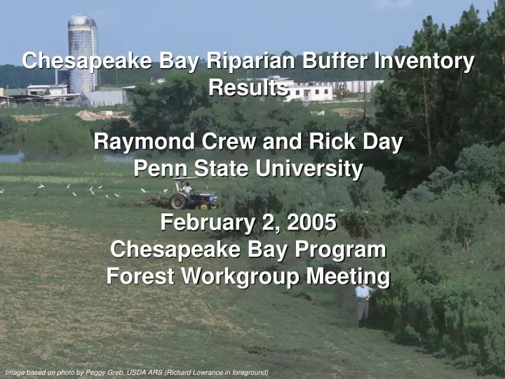
Chesapeake Bay Riparian Buffer Inventory Results Raymond Crew and Rick Day Penn State University February 2, 2005 Chesapeake Bay Program Forest Workgroup Meeting. Image based on photo by Peggy Greb, USDA ARS (Richard Lowrance in foreground). Automated Inventory Procedure.

E N D
Chesapeake Bay Riparian Buffer Inventory Results Raymond Crew and Rick DayPenn State UniversityFebruary 2, 2005Chesapeake Bay ProgramForest Workgroup Meeting Image based on photo by Peggy Greb, USDA ARS (Richard Lowrance in foreground)
Automated Inventory Procedure • determine and collect the datasets required for inventory acquire datasets • land cover • streams and water body polygons • watershed divides • calculate the inventory using an automated method • 100 and 300 foot buffers • one sided and two sided • produce datasets of the inventory useable by others
Streams and Water Body Data • Original plan was to use dataset being produced by a consortium lead by the USGS • 1:24K National Hydrography Dataset • Releases of the data did not meet the schedule of this project • Only about 70% of the Chesapeake Bay was finished in time • Solution: Use a mix of NHD data and a dataset made by the CBP
Stream and Water Body Mileages • For this project 232,049 KM or 144,189 miles • For the 1997 project 188,000 km or 117,500 miles
Watershed Divides • Watershed divide data provided by the CBPO • Two different sizes of watersheds: • 8 Digit Ave size = 226,000 HA • 11 DigitAve size = 22,000 HA
Land Cover Data • Original plan: • Have the Mid-Atlantic Regional Earth Science Applications Center (RESAC) produce a year 1990 and 2000 dataset using the same methods and type of imagery • Unfortunately only the year 2000 data was produced • No validation of the methods used to derive the land cover classes has been made publicly available
Solution • Use the best available land cover data available for the year 2000 and the year 1992 • 2000 • Use the RESAC landcover/landuse data • 1992 • Use the Multi-Resolution Land Characteristics (MRLC) landcover data. Commonly called the NLCD
2000 Landcover Data • RESAC 2000 version 1.05 • a total of 21 land cover and use classes • 4 are pertinent to this study • forest • urban forest • wetlands • water • based on three year 2000 satellite images
1992 Landcover Data • NLCD 1992 • 18 land cover classes in the Chesapeake Bay • 3 pertinent to this study • forest • wetland • water • based on primarily early 1990’s satellite images, however, some imagery as old as 1985 was used
Problems Using These Two Datasets • Different Methods uses to derive land cover categories • example: large differences between classification of open water vs. wetlands • No urban forest category in the NLCD as in the RESAC • unsure if urban forest will be classified as forest or as something else • No publicly available validation studies on the RESAC data • NLCD based on a wider temporal range of images
Riparian Buffer Algorithm • splits streams into 300’ (91.44 m) segments • orients a transect perpendicular to each stream segment at the center of the segment • establishes sampling locations every 50 feet (15.24 m) along the transect • collects the land cover informationfrom the satellite imagery at each sample location • calculates buffer statistics for each watershed • 100’ and 300’ • One side, both sides • for forest, forest & wetlands
Why not typical polygon buffers? • Would not provide statistics on contiguous land cover • Could split the polygons every linear 300 feet and at 50 foot intervals • However the resulting dataset would be much larger than the data produced by this method
Statistics being Reported • One or more sides buffered 100 feet or more • One or more sides buffered 300 feet or more • Both sides buffered 100 feet of more • Both sides buffered 300 feet or more
Statistics being Reported • Multiple types of buffer conditions: • forest • forest or urban forest • forest or urban forest or wetlands • forest or urban forest or wetlands or water n.b. no urban forest breakdown possible for 1992 Inventory
Statistics being Reported • At multiple geographic scales • 11 digit watersheds • 8 digit watersheds • for the entire Chesapeake Bay • For each of the States and the District of Columbia
2000 Inventory - forested - at least 100 Feet - both sides
1992 Inventory - forested - at least 100 Feet - both sides
2000 Inventory - forest, wetland or water - at least 100 Feet - both sides
1992 Inventory - forest, wetland or water - at least 100 Feet - both sides