Download
1 / 75
750 likes | 899 Vues
HW #7 ANSWER 17.2-3 17.5-1 17.5-9. 17.2-3 (a). A parking lot is a queueing system for providing cars with parking opportunities. The parking spaces are servers. The service time is the amount of time a car spends in a system. The queue capacity is 0. (b). (c). 17.5-1 (a). 3. 2.

E N D
HW #7 ANSWER 17.2-3 17.5-1 17.5-9
17.2-3 (a) A parking lot is a queueing system for providing cars with parking opportunities. The parking spaces are servers. The service time is the amount of time a car spends in a system. The queue capacity is 0.
(b) (c)
17.5-1 (a) 3 2 1 0 . . . 4 0 1 2 3 2 2 2 2
17.5-9 (a) . . . 0 1 2 3
How do companies use operations research to improve their inventor policy? 1. Formulate a mathematical model describing the behavior of the inventory system. 2. Seek an optimal inventory policy with respect to this model.
3. Use a computerized information processing system to maintain a record of the current inventory levels. 4. Using this record of current inventory levels, apply the optimal inventory policy to signal when and how much to replenish inventory.
The mathematical inventory models can be divided into two broad categories, (a) Deterministic models (b) Stochastic models according to the predictability of demand involved. The demand for a product in inventory is the number of units that will need to be withdrawn from inventory for some use during a specific period.
Components of Inventory Models Some of the costs that determine this profitability are (1) ordering costs, (2) holding costs, (3) Shortage costs. Other relevant factors include (4) revenues, (5) salvage costs, (6) discount rates.
The cost of ordering can be represented by a function c(z). cost of ordering z units Where K = setup cost and c = unit cost.
(2) The holding cost (sometimes called the storage cost) represents all the associated with the storage of the inventory until it is sold or used. The holding cost can be assessed either continuously or on a period-by-period basis.
(3) The shortage cost (sometimes called the unsatisfied demand cost) is incurred when the amount of the commodity required (demand) exceeds the available stock.
The criterion of minimizing the total (expected) discounted cost. A useful criterion is to keep the inventory policy simple, i.e., keep the rule for indicating when to order and how much to order both understandable and easy to implement.
Lead Time: The lead time, which is the amount of time between the placement of an order to replenish inventory and the receipt of the goods into inventory. If the lead time always is the same (a fixed lead time), then the replenishment can be scheduled just when desired.
Deterministic Continuous-Review Models A simple model representing the most common inventory situation faced by manufacturers, retailers, and wholesalers is the EOQ (Economic Order Quantity) model. (It sometimes is also referred to as the economic lot-size model.)
Inventory level Batch size Time The EOQ Model
The Basic EOQ Model Assumptions (Basic BOQ Model): 1. A known constant demand rate of a units per unit time. 2. The order quantity (Q) to replenish inventory arrives all at once just when desired, namely, when the inventory level drops to 0. 3. Planned shortages are not allowed.
K = setup cost for ordering one batch, c = unit cost for producing or purchasing each unit, h = holding cost per unit per unit of time held in inventory. The objective is to determine when and how much to replenish inventory so as to minimize the total cost.
The inventory level at which the order is placed is called the reorder point. The time between consecutive replenishments of inventory is referred to as a cycle. In general, a cycle length is Q/a.
The total cost per unit time T : Production or ordering cost per cycle = K + cQ. Average inventory level = (Q + 0)/2 = Q/2 units, Average holding cost = hQ/2 per unit time. Cycle length = Q/a, Holding cost per cycle = Total cost per cycle = The total cost per unit is
The value of Q, say Q*, that minimizes T is found by setting the first derivative to zero. so that which is well-known EOQ formula. The corresponding cycle time, say t*, is
As the setup cost K increases, both Q* and t* increase (fewer setups). When the unit holding cost h increases, both Q* and t* decrease (smaller inventory levels). As the demand rate a increases, Q* increases (larger batches) but t* decreases (more frequent setups).
The EOQ Model with Planned Shortages Planned shortages now are allowed. When a shortage occurs, the affected customers will wait for the product to become available again. Their backorders are filled immediately when the order quantity arrives to replenish inventory.
The inventory levels extend down to negative values that reflect the number of units of the product that are backordered. Inventory level Batch size Time The EOQ Model with Planned Shortages
Let p = shortage cost per unit short per unit of time short. S = inventory level just after a batch of Q units is added. Q - S = shortage in inventory just before a batch of Q units is added. The total cost per unit time is obtained from the following components. Production or ordering cost per cycle = K + cQ.
During each cycle, the inventory level is positive for a time S/a. The average inventory level during this time is (S + 0)/2 = S/2 units, and the corresponding cost is hS/2 per unit time. Hence, Holding cost per cycle =
Similarly, shortage occur for a time (Q - S)/a. The average amount of shortages during this time is (0 + Q - S)/2 =(Q - S)/2 units, and the corresponding cost is p(Q - S)/2 per unit time. Shortage cost per cycle
Therefore, Total cost per cycle and the total cost per unit time is
There are two decision variables (S and Q) in this model, so the optimal values (S* and Q*) are found by setting = = 0 Solving these equations simultaneously leads to
The optimal cycle length t* is given by The maximum shortage is
The EOQ Model with Quantity Discounts The unit cost of an item now depends on the quantity in the batch. In particular, an incentive is provided to place a large order by replacing the unit cost for a small quantity by a smaller unit cost for every item in a larger batch, and perhaps by even smaller unit costs for even larger batches.
Deterministic Periodic-Review Model When the amounts that need to be withdrawn form inventory are allowed to vary from period to period, the EOQ formula no longer ensures a minimum-cost solution.
Stochastic Continuous-Review Model Stochastic Inventory models are designed for analyzing inventory systems where there is considerable uncertainty about future demands. Computerized Inventory Systems: Each addition to inventory and each sale causing a withdrawal are recorded electronically, so that the current inventory level always is in the computer.
A continuous-review inventory system for a particular product normally will be based on two critical numbers: R = reorder point. Q = Order quantity. For a manufacturer managing its finished products inventory, the order will be for a production run of size Q. For a wholesaler or retailer, the order will be a purchase order for Q units of the product.
An inventory policy based on these two critical numbers is a simple one. Inventory policy: Whenever the inventory level of the product drops to R units, place an order for Q more units to replenish the inventory. Such a policy is often called a reorder-point,order-quantity policy, or (R, Q) policy.
The Assumptions of the Model 1. Each application involves a single product. 2. The inventory level is under continuous review, so its current value always is known. 3. An (R, Q) policy is to be used, so the only decisions to be made are to choose R and Q. 4. There is a lead time between when the order is placed and when the order quantity is received. This lead time can be either fixed or variable.
5. The demand for withdrawing units from inventory to sell them during this lead time is uncertain. However, the probability distribution of demand is known. 6. If a stockout occurs before the order is received, the excess demand is backlogged, so that the backorders are filled once the order arrives. 7. A fixed setup cost (denoted by K) is incurred each time an order is placed.
8. Except for this setup cost, the cost of the order is proportional to the order quantity Q. 9. A certain holding cost (denoted by h) is incurred for each unit in inventory per unit time. 10. When a stockout occurs, a certain shortage cost (denoted by p) is incurred for each unit backordered per unit time until the backorder is filled.
Choosing the Order Quantity Q Use the formula for the EOQ model with planned shortages. Where A is the average demand per unit time, and where K, h, and p are defined in assumptions 7, 9, and 10, respectively.
Choosing the Reorder Point R A common approach to choosing the reorder point R is to base it on management’s desired level of service to customers. Thus, the starting point is to obtain a managerial decision on service level.
Alternative Measures of Service Level 1. The probability that a stockout will not occur between the time an order is placed and the order quantity is received. 2. The average number of stockout per year. 3. The average percentage of annual demand that can be satisfied immediately. 4. The average delay in filling backorders when a stockout occurs. 5. The overall average delay in filling orders
The desired level of service under this measure is denoted by L, so L = management’s desired probability that a stockout will not occur between the time an order quantity is placed and the order quantity is received. Using measure 1 involves working with the estimated probability distribution of the following random variable. D = demand during the lead time in filling an order
For example, with a uniform distribution, the formula for choosing the reorder point R is a simple one. If the probability distribution of D is a uniform distribution over the interval from a to b, set R = a + L(b - a), because then
Since the mean of this distribution is The amount of safety stock (the expected inventory level just before the order quantity is received) provided by the reorder point R is Safety stock
General Procedure for Choosing R under Service Level Measure 1 1. Choose L. 2. Solve for R such that For example, suppose that D has a normal distribution with mean and variance Given the value of L, the table for the normal distribution then can be used to determine the value of R.