Keith Riles University of Michigan

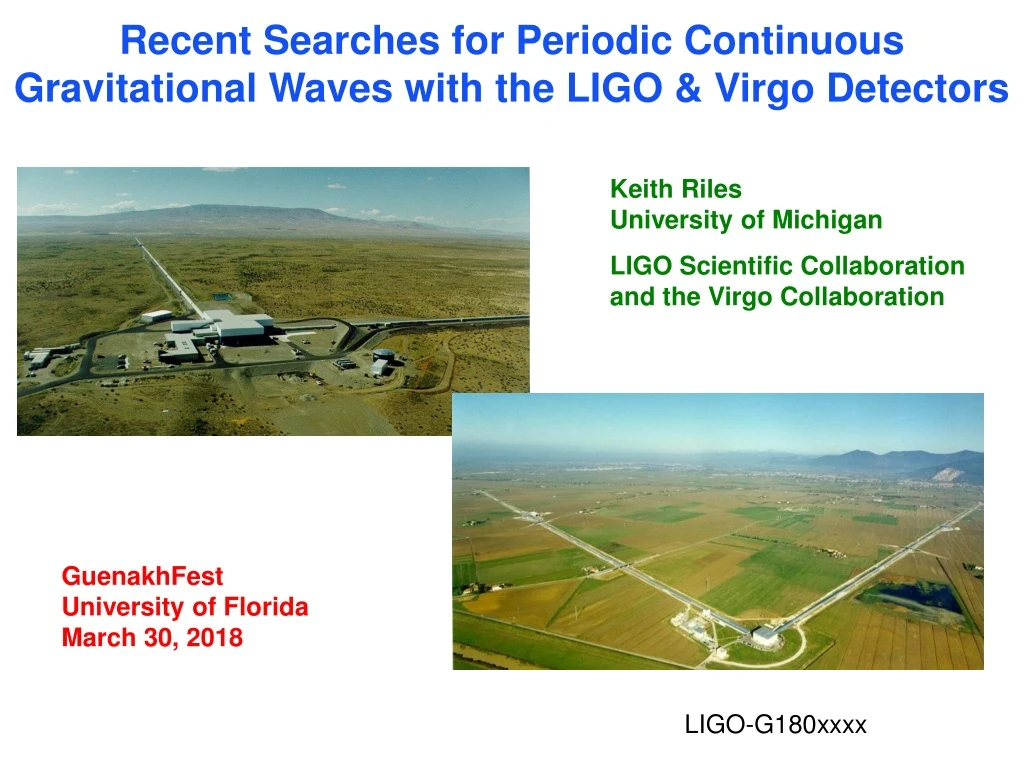
1. Recent Searches for Periodic Continuous Gravitational Waves with the LIGO & Virgo Detectors Keith Riles University of Michigan LIGO Scientific Collaboration and the Virgo Collaboration GuenakhFest University of Florida March 30, 2018 LIGO-G180xxxx

2. Generation of Continuous Gravitational Waves • Radiation generated by quadrupolar mass movements: (Iμν = quadrupole tensor, r = source distance) No GW from axisymmetric object rotating about symmetry axis • Spinning neutron star with equatorial ellipticity εequat Courtesy: U. Liverpool gives a strain amplitude h(fGW = 2fRot):

3. Gravitational CW mechanisms • Equatorial ellipticity (e.g., – mm-high “bulge”): • Poloidal ellipticity (natural) + wobble angle (precessing star): (precession due to differentLand Ωaxes) • Two-component (crust+superfluid)  • r modes (rotational oscillations – CFS-driven instability): • N. Andersson, ApJ 502 (1998) 708 • S. Chandrasekhar PRL 24 (1970) 611 • J. Friedman, B.F. Schutz, ApJ 221 (1978) 937

4. Gravitational CW mechanisms • Assumption we (LSC, Virgo) have usually made to date: • Bulge is best bet for detection •  Look for GW emission at twice the EM frequency • e.g., look for Crab Pulsar (29.7 Hz) at 59.5 Hz • (troublesome frequency in North America!) What is allowed for εequat ? Old maximum (?) ≈ 5 × 10-7[σ/10-2] (“ordinary” neutron star) with σ = breaking strain of crust G. Ushomirsky, C. Cutler, L. Bildsten MNRAS 319 (2000) 902 More recent finding: σ≈ 10-1 supported by detailed numerical simulation C.J. Horowitz & K. Kadau PRL 102, (2009) 191102 Recent re-evaluation: εequat< 10-5 N.K. Johnson-McDaniel & B.J. Owen PRD 88 (2013) 044004

5. Gravitational CW mechanisms Strange quark stars could support much higher ellipticities B.J. Owen PRL 95 (2005) 211101, Johnson-McDaniel & Owen (2013) Maximum εequat≈ 10-1 (!) But what εequat is realistic? What could drive εequat to a high value (besides accretion)? Millisecond pulsars have spindown-implied values lower than 10-9–10-6 New papers revisiting possible GW emission mechanisms (e.g., buried magnetic fields, accretion-driven r-modes) are also intriguing

6. Finding a completely unknown CW Source Serious technical difficulty: Doppler frequency shifts • Frequency modulation from earth’s rotation (v/c ~ 10-6) • Frequency modulation from earth’s orbital motion (v/c ~ 10-4) • Coherent integration of 1 year gives frequency resolution of 30 nHz • 1 kHz source spread over 6 million bins in ordinary FFT! Additional, related complications: • Daily amplitude modulation of antenna pattern • Spin-down of source • Orbital motion of sources in binary systems

7. Finding a completely unknown CW Source Modulations / drifts complicate analysis enormously: • Simple Fourier transform inadequate • Every sky direction requires different demodulation Computational scaling: Single coherence time – Sensitivity improves as (Tcoherence)1/2 but cost scales with (Tcoherence)6+  Restricts Tcoherence < 1-2 days for all-sky search  Exploit coincidence among different spans Alternative: Semi-coherent stacking of spectra (e.g., Tcoherence = 30 min)  Sensitivity improves only as (Nstack)1/4  All-sky survey at full sensitivity = Formidable challenge • Impossible?

8. But three substantial benefits from modulations: • Reality of signal confirmed by need for corrections • Corrections give precise direction of source • Single interferometer can make definitive discovery Can “zoom in” further with follow-up algorithms once we lock on to source Sky map of strain power for signal injection (semi-coherent search) [V. Dergachev, PRD 85 (2012) 062003 M. Shaltev & R. Prix, PRD 87 (2013) 084057]

9. Recent results Targeted search for 200 known pulsars in O1 data • Lowest (best) upper limit on strain: • h0 < 1.6 × 10−26 • Lowest (best) upper limit on ellipticity: • ε < 1.3 × 10-8 • Crab limit at 0.2% of total energy loss Journal ref arXiv:1309.4027 (Sept 2013)

10. Another take on the 200* *Also looked for non-tensorial polarizations – none seen (PRD ….)

11. Recent results – Narrowband Search Journal ref Add explanatory text with highlights

12. Recent results – Scorpius X-1 Journal ref

13. Recent results – All-sky search Journal ref

14. Recent results – All-sky search Journal ref

15. Recent results – All-sky search Journal ref

16. Summary • No CW discoveries yet, but… • Still examining data we have taken in O2 run • Future: • More sensitive detectors • Longer (and cleaner) data sets • Improved algorithms • Could be on cusp of new type of GW discovery • Nature sometimes bestows golden gifts…

17. Extra Slides

18. Other results Not all known sources have measured timing • Compact central object in the Cassiopeia A supernova remnant • Birth observed in 1681 – One of the youngest neutron stars known • Star is observed in X-rays, but no pulsations observed • Requires a broad band search over accessible band Cassiopeia A

19. Other results Search for Cassiopeia A – Young age (~300 years) requires search over 2nd derivative indirect upper limit (based on age, distance) Ap. J. 722 (2010) 1504

20. Other results S5 all-sky results: Semi-coherent stacks of 30-minute, demodulated power spectra (“PowerFlux”) Astrophysical reach: PRD 85 (2012) 022001

21. Other results Einstein@Home semi-coherent sums of 121 25-hour F-Statistic powers (2 interferometers) S5 all-sky results: Astrophysical reach: PRD 87 (2013) 042001

22. Other results Hough-transform search based on ~68K 30-minute demodulated spectra (3 interferometers) S5 all-sky results: arXiv:1311.2409 (Nov 2013)

23. GEO-600 Hannover • LIGO Hanford • LIGO Livingston • Current search point • Current search coordinates • Known pulsars • Known supernovae remnants http://www.einsteinathome.org/ Your computer can help too!

24. Frequency Time Time Searching for continuous waves Several approaches tried or in development: • Summed powers from many short (30-minute) FFTs with sky-dependent corrections for Doppler frequency shifts  “Semi-coherent “ • (StackSlide, Hough transform (2 types), PowerFlux) • Push up close to longest coherence time allowed by computing resources (~few days) and look for coincidences among outliers in different data stretches (demodulation-based F-Statistic) Frequency bin

25. What is the “direct spindown limit”? It is useful to define the “direct spindown limit” for a known pulsar, under the assumption that it is a “gravitar”, i.e., a star spinning down due to gravitational wave energy loss Unrealistic for known stars, but serves as a useful benchmark Equating “measured” rotational energy loss (from measured period increase and reasonable moment of inertia) to GW emission gives: • Example: • Crab hSD = 1.4 × 10-24 • (d=2 kpc, fGW = 59.5 Hz, dfGW/dt = −7.4×10-10 Hz/s )

26. What is the “indirect spindown limit”? If a star’s age is known (e.g., historical SNR), but its spin is unknown, one can still define an indirect spindown upper limit by assuming gravitar behavior has dominated its lifetime: And substitute into hSD to obtain [K. Wette, B. Owen,… CQG 25 (2008) 235011] • Example: • Cassiopeia A hISD = 1.2 × 10-24 • (d=3.4 kpc, τ=328 yr)

27. What is the “X-ray flux limit”? For an LMXB, equating accretion rate torque (inferred from X-ray luminosity) to gravitational wave angular momentum loss (steady state) gives: [R.V. Wagoner ApJ 278 (1984) 345; J. Papaloizou & J.E. Pringle MNRAS 184 (1978) 501; L. Bildsten ApJ 501 (1998) L89] • Example: Scorpius X-1 •  hX-ray≈ 3 × 10-26[600 Hz / fsig]1/2 • (Fx= 2.5 × 10-7 erg·cm-2·s-1) Courtesy: McGill U.