A BIONETGEN Tutorial
A BIONETGEN Tutorial. Outline. Downloading BNG Installing BNG Running BNG text-based interface graphical interface – RULEBUILDER web-based interface – GETBONNIE Simple example Extending the example Detailed model of TLR4 signaling. Creating a BNG model.


A BIONETGEN Tutorial
E N D
Presentation Transcript
Outline • Downloading BNG • Installing BNG • Running BNG • text-based interface • graphical interface – RULEBUILDER • web-based interface – GETBONNIE • Simple example • Extending the example • Detailed model of TLR4 signaling
Creating a BNG model 6. Create a BioNetGen model (with .bngl extension) in a text file using your favorite editor.
Running BNG 7. Open a terminal window, navigate to the file location, and type path to BNG2.pl followed by filename.
The BNG logfile 8. (optional) Piping output to a logfile. ~/BioNetGen2/Perl2/BNG2.pl example1.bngl > & example1.log BioNetGen version 2.0.48 readFile::Reading from file example1.bngl Read 11 parameters. Read 3 species. Adding P as allowed state of component Y of molecule R Read 3 observable(s). Read 5 reaction rule(s). Iteration 0: 3 species 0 rxns 0.00e+00 CPU s Iteration 1: 4 species 1 rxns 1.00e-02 CPU s Iteration 2: 5 species 3 rxns 0.00e+00 CPU s Iteration 3: 6 species 5 rxns 1.00e-02 CPU s Iteration 4: 9 species 9 rxns 1.00e-02 CPU s Iteration 5: 12 species 20 rxns 3.00e-02 CPU s Iteration 6: 14 species 32 rxns 3.00e-02 CPU s Iteration 7: 14 species 36 rxns 2.00e-02 CPU s Cumulative CPU time for each rule Rule 1: 6 reactions 3.00e-02 CPU s 5.00e-03 CPU s/rxn Rule 2: 12 reactions 5.00e-02 CPU s 4.17e-03 CPU s/rxn Rule 3: 3 reactions 0.00e+00 CPU s 0.00e+00 CPU s/rxn Rule 4: 5 reactions 2.00e-02 CPU s 4.00e-03 CPU s/rxn Rule 5: 10 reactions 1.00e-02 CPU s 1.00e-03 CPU s/rxn Total : 36 reactions 1.10e-01 CPU s 3.06e-03 CPU s/rxn Wrote network to example1.net. CPU TIME: generate_network 0.1 s. Network simulation using ODEs Running run_network on phoebe
Overview of inputs and outputs NETWORK .cdat BNGL ODE BIONETGEN .net SSA .gdat .log
Elements of a BNGL file • parameters • molecule types • seed species • reaction rules • observables • actions
A simple example:Ligand-receptor binding EGF Vo V EGFR
A simple example:parameters begin parameters # Physical and geometric constants NA 6.0e23 #Avogadro’s num f 1 #scaling factor Vo f*1e-10 # L V f*3e-12 # L # Initial concentrations EGF0 2e-9*NA*Vo #nM EGFR0 f*1.8e5 #copy per cell # Rate constants kp1 9.0e7/(NA*Vo) #input /M/sec km1 0.06 #/sec end parameters EGF Vo V EGFR
A simple example:parameters • Summary • Concentration units : copies per cell • Multiply concentrations by NA*Vrxn • Don’t scale first order rate constants • Divide second order rate constants by NA*Vrxn • Following this recipe allows switching between ODE and stochastic simulation without parameter modification. EGF Vo V EGFR
A simple example:molecule types R begin molecule types EGF(R) EGFR(L,CR1,Y1068~U~P) end molecule types EGF L CR1 U Y1068 P EGFR
A simple example:seed species R begin seed species EGF(R) EGF0 EGFR(L,CR1,Y1068~U) EGFR0 end seed species EGF EGF L CR1 Y1068~U EGFR EGFR
Pattern basics Basic Definition: A set of molecules that may be partially specified and selects a set of species through its allowed mappings. EGF(R) EGFR(L) Pattern Mapping Species EGF(R) EGFR(L,CR1,Y1068~U) EGFR(L,CR1,Y1068~P)
A simple example:reaction rules k+1 + k-1 EGF EGF EGF EGF EGFR EGFR begin reaction rules EGF(R) + EGFR(L) <-> EGF(R!1).EGFR(L!1) kp1, km1 end reaction rules
A simple example:actions begin parameters … end parameters begin molecule types EGF(R) EGFR(L,CR1,Y1068~U~P) end molecule types begin seed species EGF(R) EGF0 EGFR(L,CR1,Y1068~U) EGFR0 end seed species begin reaction rules EGF(R) + EGFR(L) <-> EGF(R!1).EGFR(L!1) kp1, km1 end reaction rules # actions generate_network({overwrite=>1}); Generates network of species and reactions by iterative application of rules starting with seed species
A simple example:Application of the forward binding rule Reaction rule EGF(R) + EGFR(L) -> EGF(R!1).EGFR(L!1) kp1 Add bond Step 1: Match patterns onto reactant species. Step 2: Copy selected species to product side. Step 3: Apply transformation specified by rule.
A simple example:Application of the forward binding rule Reaction rule EGF(R) + EGFR(L) -> EGF(R!1).EGFR(L!1) kp1 Add bond Step 1: Match patterns onto reactant species. + EGF(R) EGFR(L,CR1,Y1068~U)
A simple example:Application of the forward binding rule Reaction rule EGF(R) + EGFR(L) -> EGF(R!1).EGFR(L!1) kp1 Add bond Step 1: Match patterns onto reactant species. + EGF(R) EGFR(L,CR1,Y1068~U) Step 2: Copy selected species to product side. -> EGF(R) + EGFR(L,CR1,Y1068~U)
A simple example:Application of the forward binding rule Reaction rule EGF(R) + EGFR(L) -> EGF(R!1).EGFR(L!1) kp1 Add bond Step 1: Match patterns onto reactant species. + EGF(R) EGFR(L,CR1,Y1068~U) Step 2: Copy selected species to product side. -> EGF(R) + EGFR(L,CR1,Y1068~U) Step 3: Apply transformation specified by rule. -> EGF(R!1).EGFR(L!1,CR1,Y1068~U) kp1 New species
A simple example:Application of the forward binding rule Reaction rule EGF(R) + EGFR(L) -> EGF(R!1).EGFR(L!1) kp1 Add bond + EGF(R) EGFR(L,CR1,Y1068~U) -> EGF(R!1).EGFR(L!1,CR1,Y1068~U) kp1 New species New reaction
A simple example:Application of the reverse binding rule Reaction rule EGF(R!1).EGFR(L!1) -> EGF(R) + EGFR(L) km1 Delete bond EGF(R!1).EGFR(L!1,CR1,Y1068~U)
A simple example:Application of the reverse binding rule Reaction rule EGF(R!1).EGFR(L!1) -> EGF(R) + EGFR(L) km1 Delete bond EGF(R!1).EGFR(L!1,CR1,Y1068~U) -> EGF(R!1).EGFR(L!1,CR1,Y1068~U)
A simple example:Application of the reverse binding rule Reaction rule EGF(R!1).EGFR(L!1) -> EGF(R) + EGFR(L) km1 Delete bond EGF(R!1).EGFR(L!1,CR1,Y1068~U) -> EGF(R) + EGFR(L,CR1,Y1068~U) km1 New reaction2
A simple example: Overview of generate_network seed species EGF(R) EGFR(L,CR1,Y1068~U) Iteration 1: rule1f: EGF(R) + EGFR(L) -> EGF(R!1).EGFR(L!1) kp1
A simple example: Overview of generate_network seed species EGF(R) EGFR(L,CR1,Y1068~U) Iteration 1: rule1f: EGF(R) + EGFR(L) -> EGF(R!1).EGFR(L!1) kp1 new reaction: EGF(R) + EGFR(L,CR1,Y1068~U) -> EGF(R!1).EGFR(L!1,CR1,Y1068~U) kp1 new species: EGF(R!1).EGFR(L!1,CR1,Y1068~U)
A simple example: Overview of generate_network seed species EGF(R) EGFR(L,CR1,Y1068~U) Iteration 1: rule1f: EGF(R) + EGFR(L) -> EGF(R!1).EGFR(L!1) kp1 new reaction: EGF(R) + EGFR(L,CR1,Y1068~U) -> EGF(R!1).EGFR(L!1,CR1,Y1068~U) kp1 new species: EGF(R!1).EGFR(L!1,CR1,Y1068~U) Network after Iteration 1 species 1 EGF(R) 2 EGFR(L,CR1,Y1068~U) 3 EGF(R!1).EGFR(L!1,CR1,Y1068~U) reactions 1 1,2 3 kp1
A simple example: Overview of generate_network From iteration 1 species 1 EGF(R) 2 EGFR(L,CR1,Y1068~U) 3 EGF(R!1).EGFR(L!1,CR1,Y1068~U) Iteration 2: rule1r: EGF(R!1).EGFR(L!1) -> EGF(R) + EGFR(L) km1 new reaction: EGF(R!1).EGFR(L!1,CR1,Y1068~U) -> EGF(R) + EGFR(L,CR1,Y1068~U) km1 Network after Iteration 2 species 1 EGF(R) 2 EGFR(L,CR1,Y1068~U) 3 EGF(R!1).EGFR(L!1,CR1,Y1068~U) reactions 1 1,2 3 kp1 # rule1f 2 3 1,2 km1 # rule1r
A simple example: Overview of generate_network From iteration 1 species 1 EGF(R) 2 EGFR(L,CR1,Y1068~U) 3 EGF(R!1).EGFR(L!1,CR1,Y1068~U) Iteration 2: rule1r: EGF(R!1).EGFR(L!1) -> EGF(R) + EGFR(L) km1 new reaction: EGF(R!1).EGFR(L!1,CR1,Y1068~U) -> EGF(R) + EGFR(L,CR1,Y1068~U) km1 Network after Iteration 2 - final species 1 EGF(R) 2 EGFR(L,CR1,Y1068~U) 3 EGF(R!1).EGFR(L!1,CR1,Y1068~U) reactions 1 1,2 3 kp1 # rule1f 2 3 1,2 km1 # rule1r
A simple example: Running BNG2.pl BNGL generate_network .net BNG2.pl .log
A simple example: Running BNG2.pl phoebe% ~/BioNetGen2/Perl2/BNG2.pl SimpleExample.bngl /Users/faeder/BioNetGen2/Perl2/BNG2.pl BioNetGen version 2.0.48 readFile::Reading from file SimpleExample.bngl Read 8 parameters. Read 2 molecule types. Read 2 species. Read 1 reaction rule(s). WARNING: Removing old network file SimpleExample.net. Iteration 0: 2 species 0 rxns 0.00e+00 CPU s Iteration 1: 3 species 1 rxns 0.00e+00 CPU s Iteration 2: 3 species 2 rxns 0.00e+00 CPU s Cumulative CPU time for each rule Rule 1: 2 reactions 0.00e+00 CPU s 0.00e+00 CPU s/rxn Total : 2 reactions 0.00e+00 CPU s 0.00e+00 CPU s/rxn Wrote network to SimpleExample.net.
A simple example:The .net file begin molecule types 1 EGF(R) 2 EGFR(L,CR1,Y1068~U~P) end molecule types begin species 1 EGF(R) EGF0 2 EGFR(CR1,L,Y1068~U) EGFR0 3 EGF(R!1).EGFR(CR1,L!1,Y1068~U) 0 end species begin reaction rules Rule1: \ EGF(R) + EGFR(L) <-> EGF(R!1).EGFR(L!1) kp1, km1 # Bind(0.0.0,0.1.0) # Reverse # Unbind(0.0.0,0.1.0) end reaction rules begin reactions 1 1,2 3 kp1 #Rule1 2 3 1,2 km1 #Rule1r end reactions The .netfile SimpleExample.net
Translation of the network model into ordinary differential equations species 1 EGF(R) EGF0 2 EGFR(CR1,L,Y1068~U) EGFR0 3 EGF(R!1).EGFR(CR1,L!1,Y1068~U) 0 Dependent variables reactions 1 1,2 3 kp1 #Rule1 2 3 1,2 km1 #Rule1r Flux terms f1 f2
Exporting the model BNGL generate_network .net BNG2.pl writeformat M-file SBML .log
Exporting model equations to Matlab:writeMfile begin parameters … end parameters begin molecule types EGF(R) EGFR(L,CR1,Y1068~U~P) end molecule types begin seed species EGF(R) EGF0 EGFR(L,CR1,Y1068~U) EGFR0 end seed species begin reaction rules EGF(R) + EGFR(L) <-> EGF(R!1).EGFR(L!1) kp1, km1 end reaction rules # actions generate_network({overwrite=>1}); writeMfile();
Ordinary differential equations in the M-file SimpleExample.m % M-file for model SimpleExample created by BioNetGen 2.0.48 function [t_out,obs_out,x_out]= SimpleExample(tend) Nspecies=3; Nreactions=2; obs_out=zeros(1); % Parameters NA=6.0e23; f=1; Vo=f*1e-10; V=f*3e-12; EGF0=(2e-9*NA)*Vo; EGFR0=f*1.8e5; kp1=3.0e6/(NA*V); km1=0.06; % Intial concentrations x0= [ EGF0; EGFR0; 0;]; % Reaction flux function function f= flux(t,x) f(1)=kp1*x(1)*x(2); f(2)=km1*x(3); end % Derivative function function d= xdot(t,x) f=flux(t,x); d(1,1)= -f(1) +f(2); d(2,1)= -f(1) +f(2); d(3,1)= +f(1) -f(2); end snames={'EGF(R)','EGFR(CR1,L,Y1068~U)','EGF(R!1).EGFR(CR1,L!1,Y1068~U)'}; % Integrate ODEs [t_out,x_out]= ode15s(@xdot, [0 tend], x0); % plot species concentrations plot(t_out,x_out); legend(snames); end
Running exported model as a Matlab function >> SimpleExample(120)
Export to the Systems Biology Markup Language (SBML) • SBML is an XML specification for biological models • Many simulation tools read and write SBML • Supports standard reaction network models • generate_network must be invoked prior to export • Support for rule-based models will appear in Level 3 (current level is 2+) • Website: http://sbml.org
Running the simulation within BioNetGen NETWORK .cdat generate_network simulate_ode BNGL ODE BNG2.pl .net SSA .gdat simulate_ssa .log
Running the simulation within BioNetGen begin parameters … end parameters begin molecule types EGF(R) EGFR(L,CR1,Y1068~U~P) end molecule types begin seed species EGF(R) EGF0 EGFR(L,CR1,Y1068~U) EGFR0 end seed species begin reaction rules EGF(R) + EGFR(L) <-> EGF(R!1).EGFR(L!1) kp1, km1 end reaction rules # actions generate_network({overwrite=>1}); saveConcentrations(); simulate_ode({suffix=>ode,t_end=>120,n_steps=>50});
Running the simulation within BioNetGen begin parameters … end parameters begin molecule types EGF(R) EGFR(L,CR1,Y1068~U~P) end molecule types begin seed species EGF(R) EGF0 EGFR(L,CR1,Y1068~U) EGFR0 end seed species begin reaction rules EGF(R) + EGFR(L) <-> EGF(R!1).EGFR(L!1) kp1, km1 end reaction rules # actions generate_network({overwrite=>1}); saveConcentrations(); simulate_ode({suffix=>ode,t_end=>120,n_steps=>50}); BNG, like many other systems biology applications, uses the CVODE library for solving ODE’s. Sparse option can be used to solve systems up to about 50,000 equations.
The .cdat file SimpleExample_ode.cdat # time 1 2 3 0.0000000000000000e+00 1.2000000000000000e+05 1.8000000000000000e+05 0.0000000000000000e+00 2.3999999999999999e+00 6.9387285118773594e+04 1.2938728511877365e+05 5.0612714881226493e+04 4.7999999999999998e+00 5.0363939566816996e+04 1.1036393956681706e+05 6.9636060433183069e+04 7.1999999999999993e+00 4.1819631802026437e+04 1.0181963180202652e+05 7.8180368197973614e+04 Your favorite plotting package • Some useful options • PhiBPlot – Java-based (JFreeChart) plotting utility provided with BNG • xmgrace – Unix / X windows graphing package great for XY plots • Matlab, Mathematica, gnuplot, Excel, etc.
The .cdat file in PhiBPlot These numbers correspond to indices of species in .net file
The .cdat file in PhiBPlot These numbers correspond to indices of species in .net file begin species 1 EGF(R) EGF0 2 EGFR(CR1,L,Y1068~U) EGFR0 3 EGF(R!1).EGFR(CR1,L!1,Y1068~U) 0 end species
Stochastic simulations in BioNetGen • Network simulation engine uses Gillespie Direct method • Adequate performance for networks with up to ~50,000 species. • May be used in ‘on-the-fly’ mode, which generates species and reactions as needed
Stochastic simulations in BioNetGen • Network simulation engine uses Gillespie Direct method • Adequate performance for networks with up to ~50,000 species. • May be used in ‘on-the-fly’ mode, which generates species and reactions as needed
Comparison between ODE and stochastic simulations begin parameters … end parameters begin molecule types EGF(R) EGFR(L,CR1,Y1068~U~P) end molecule types begin seed species EGF(R) EGF0 EGFR(L,CR1,Y1068~U) EGFR0 end seed species begin reaction rules EGF(R) + EGFR(L) <-> EGF(R!1).EGFR(L!1) kp1, km1 end reaction rules # actions generate_network({overwrite=>1}); saveConcentrations(); simulate_ode({suffix=>ode,t_end=>120,n_steps=>50}); resetConcentrations(); simulate_ssa({suffix=>ssa,t_end=>120,n_steps=>50});
Viewing comparison in PhiBPlot Noise is minimal because species concentrations are high.