Download
1 / 43
430 likes | 647 Vues
GLY 521 Hydrogeophysics. Upland Recharge to a Valley Fill Aquifer. After Frimpter, 1978. Elastic Waves

E N D
Elastic Waves Elastic Behavior -- the ability of a material to immediately return to its original size, shape, or position after being squeezed, stretched, or otherwise deformed. The material follows Hooke’s Law (s = Ce). Plastic (Ductile) Behavior -- a permanent change in the shape, size, etc., of a solid that does not involve failure by rupture. Stress -- force per unit area (s) Strain -- change in shape or size (e)
Elastic Waves So in general, all seismic waves are elastic waves and propagate through material through elastic deformation. We can design computer models of earth materials to behave elastically, and demonstrate not only how seismic waves propagate, but also the form in which they propagate. The following models plot in color the displacement of material as seismic energy passes.
Elastic Waves, as waves in general, can be described spatially...
Elastic Waves The controlling factors in the propagation of seismic wave are the physical properties of the material through which the seismic energy is travelling. The specific properties are called the elastic constants: Bulk Modulus (k) -- describes the ability to resist being compressed. Shear Modulus (µ) -- describes the ability to resist shearing.
Elastic Waves It turns out that k and µ can be difficult to measure, so other elastic constants relating the two were derived: Young’s Modulus (E) -- describes longitudinal strain in a body subjected to longitudinal stress. Poisson’s Ratio (n) -- describes transverse strain divided by longitudinal strain in a body subjected to longitudinal stress.
Elastic Waves Leme’s Constant (l) -- interrelates all four elastic constants and is very useful in mathematical computations, though it doesn’t have a good intuitive meaning. l = k - 2m = n E 3 (1 + n)(1-2 n) It’s important for you to know the terms and what they represent (when appropriate) because we will be using them in labs.
The Wave Equation We’ll look at the scalar wave equation to mathematically express how elastic strain (dilatation, D) propagates through a material: rd2D = (l + 2m) 2Ddt2 where D = exx + eyy + ezz and 2 is the Lapacian of D, or d2D/dx2 + d2D/dy2 + d2D/dz2 D D
Elastic Waves When solving the wave equation (which describes how energy propagates through an elastic material), there are two solutions that solve the equation, Vp and Vs . These solutions relate to our elastic constants by the following equations:
Elastic Waves It turns out that Vp and Vs are probably familiar to you from your introductory earthquake knowledge, since they are the velocities of P-waves and S-waves, respectively. So, now you know why there are P- and S-waves--because they are two solutions that both solve the wave equation for elastic media. S P
The Wave Equation The wave equation can be rewritten as 1 d2D = 2Da2dt2 where a2 = (l + 2m)/r, or alternatively as 1 d2Q = 2Qb2dt2 where b2 = m/r And you’ll recognize the physical realization of these equations as a = P-wave and b = S-wave velocity. D D
The Wave Equation Since the elastic constants are always positive, a is always greater than b, and b/a = [m/(l+2m)]1/2 = [(0.5-s)/(1-s)]1/2 So, as Poisson’s ratio, s, decreases from 0.5 to 0, b/a increases from 0 to it’s maximum value 1/√2; thus, S-wave velocity must range from 0 to 70% of the P-wave velocity of any material.
The Wave Equation Modeled As displacements propagate away from the initial source of displacement (i.e., the source), a spherical wavefront is observed. Seismologists define raypaths showing the direction of propagation away from the source. Raypaths are always perpendicular to the wavefront, analogous to flowpaths in hydrology.
The Wave Equation Modeled Boundary Conditions: We’ve seen how body-wave displacements propagate through a homogeneous material, but what happens at boundaries? At boundaries (defined as a place where material elastic properties change), body waves refract (following Snell’s Law) and reflect. * Without going into details, the potential ENERGY expressed in the propagating displacements is partitioned at every interface into REFRACTED (or transmitted) and REFLECTED energy as stated by the complex Zoeppritz Equations.
The Wave Equation Modeled Boundary Conditions–REFRACTION: Snell’s Law states that an incident raypath will refract at an interface to a degree related to the difference in velocities:
The Wave Equation Modeled Boundary Conditions–REFRACTION: Note that by definition, if the propagation velocity increases across an interface, the ray will refract toward the interface. In the example below, the diagram is drawn such that v2 > v1.
The Wave Equation Modeled Boundary Conditions–REFLECTION: At an interface, body wave displacements also reflect. Simply, waves reflect at an interface with an angle equal to the incidence angle, regardless of the propagation velocities of the layers: i2 i1 i1 = i2
The Wave Equation Modeled So, at any interface, some energy is reflected (at the angle of incidence) and some is refracted (according to Snell’s Law). Let’s look at a simple model and just watch what happens to the P-wave energy...
The Wave Equation Modeled FYI, if we used the same model, but only looked at the surface waves, not surprisingly we would just see them move out from the source at a constant velocity.
The Wave Equation Modeled Each of the things labeled is called a phase. Phases, in layman's terms, represent a part of the original source energy that has done something.
The Wave Equation Modeled One thing we didn’t check out is what happens when the variables are set up just right so that i2 = 90°. That means the energy will travel right along the interface. It turns out that this phenomenon generates the interesting head wave phase. An important term to know is critical angle. The critical angle (ic)is the incidence angle at which the energy refracts directly along the interface.
The Wave Equation Modeled Head waves are generated by energy refracting along an interface, and along the way “leaking” some energy back toward the surface at the critical angle.
The Wave Equation Modeled As displacements propagate away from the initial source of displacement (i.e., the source), a spherical wavefront is observed. Seismologists define raypaths showing the direction of propagation away from the source. Raypaths are always perpendicular to the wavefront, analogous to flowpaths in hydrology.
The Wave Equation Modeled For a two-layer model with a flat interface, the three main P-wave arrivals are: (1) Direct Wave, (2) Refracted Wave (Head Wave), and (3) Reflected Wave.
The Wave Equation Modeled Even for models with no noise, identifying phases may be challenging. However, you can train your eye/brain to learn how to do this.
The Wave Equation Modeled You will learn to do this...
Refraction Interpretation We’ll now look specifically at refractions and discuss interpretation. First, let’s look at something beyond the two-layer case.
Multilayer Model Distance Time
Multilayer Model Distance Direct Wave 1st Layer Refraction Time 2nd Refraction 1st Reflection 2nd Reflection