Download
1 / 33
330 likes | 569 Vues
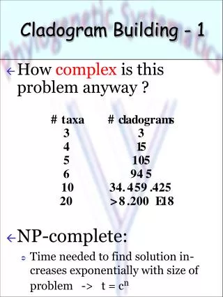
Cladogram Building - 1. How complex is this problem anyway ?. NP-complete: Time needed to find solution in-creases exponentially with size of problem -> t = c n. Computational Complexity. How do we proceed ? What about the quality of the solution ? Optimality criterion

E N D
Cladogram Building - 1 • How complex is this problem anyway ? • NP-complete: • Time needed to find solution in-creases exponentially with size of problem -> t = cn
Computational Complexity • How do we proceed ? • What about the quality of the solution? • Optimality criterion • Exact and Exhaustive • Enumeration • Branch and Bound • (maybe) Off-Target and Incomplete • Heuristics
Optimality - 1 • Parsimony analysis: • comprises a group of related methods, united by the goal of optimizingsome evolutionary significant quantity but differing in their underlying evolutionary assumptions.
Optimality - 2 • How good is the solution : • What is its score [relative to alternatives]?. • Relation of score to evolutionary assumptions • Fitch and Wagner Parsimony • Dollo Parsimony • Camin-Sokal Parsimony • Generalized Parsimony • Constrained Parsimony • Group / Component Compatibility • Character Compatibility
Exact and Exhaustive • Enumeration is computationally unfeasible if # taxa is over, say, 10. • Branch and Bound is computationally feasible for over 20 taxa (50 may even work).
(maybe) Off-Target andIncomplete • Heuristics • Step-wise Addition • Star Decomposition • Branch Swapping
A B B D B D C C A B A D C A C D E C E D C A B A B E D A D B A E A C D C B C B E Step-wise Addition - 1
Step-wise Addition - 2 • Dependent on taxon sequence in data matrix. • Excessively greedy. • Susceptible to local optima.
Branch Swapping • Local rearrangements of parts of cladogram • Nearest Neighbor Interchange • Subtree Pruning and Regrafting • Tree Bisection and Reconnection
Optimality - 3 Kind ofScores • Length (number of steps) • Consistency Index (CI) • Retention index (RI) • Corrected Extra Length (CEL) • Redundancy Quotient • AUCC • HDR • CCSI • …
Fitch & Wagner • Characters: • W: binary, ordered multistate, continuous • F: unordered multistate • Transformation: • Free reversibility • root and cladogram-length decoupled. • Change in any direction equally probable (symmetry). • W: intermediate states always involved. • Thus 1 -> 3 implies 2 steps. • F: Any state can transform into any other. • Thus 1 -> 3 implies 1 step.
A B D C E B C D E B C D E 0 2 1 3 0 2 1 3 ? ? ? 0 0 A A Wagner:Cladogram length - 1 0,2 1,3 1,2
0,2 1,3 1 1 1,2 B B B C C C D D D E E E 0 0 0 2 2 2 1 1 1 3 3 3 0 0 0 A A A Wagner:Cladogram length - 2 1 0 1 1 2 2 2 0 1 1 1
D A B E C B B C C D D E E 0 0 2 2 0 0 3 3 1 2 2 A A 1 Fitch:Cladogram length 0,2 0 1 0 0 0,3 0
A B 0 1 C 0 0 D 1 0 0 A B 0 1 C 0 E 0 D 1 E 0 Dollo:Multiple origins not allowed 1 1 1
a b c d a b c d a b c d 1 2 3 1 2 1 a b c d 1 1 1 1 1 1 a b c d A C G T a b c d M 2M 3M M 2M M A C G T 5 1 5 5 1 5 0 1 0 1 1 Generalized Parsimony Fitch Wagner 1 2 1 3 2 1 1 1 1 1 1 1 Dollo T-sition/T-version 1 2 1 3 2 1 5 1 5 5 1 5 1 Gain vs Loss
Models of Evolutionary Change • Molecular Data • Maximum Likelihood: • “Given the phylogeny, what is the probability to find the data as I did ?” • Substitution Types • Substitution Probabilities
TrN SYM HKY F84 K3ST K2P F81 Single substitution type JC Models:Substitution Types GTR T-versions; 2 T-sition class Equal base frequencies T-versions vs T-sitions T-versions; 2 T-sition class Equal base freq’s Single substitution type T-versions vs T-sitions Equal base frequencies
Substitution Types: What do they all mean ? • GTR, e.g., stands for Generalized Time Reversible, meaning that the overall rate of change from base i to base j in a given length of time is the same as the rate of change from base j to base i. • Each type corresponds to a table of substitution rates for all pairs of the nucleotides A, C, G, and T
A C G T A C G T ma mb mc mdme mf mg mh mi mj mk ml A C G T A C G T pA0 0 0 0pC0 0 0 0pG 0 0 0 0pT Substitution Rate Table • Q= R+.XÕ • pA=frequency parameter • m= mean instantaneous SR • a, … k, l = relative rate parameters. • All models can be obtained by restricting the parameters in R.
A C G T A C G T ma mb mc mdme mf mg mh mi mj mk ml A C G T A C G T pA0 0 0 0pC0 0 0 0pG 0 0 0 0pT Models:Substitution Rates • GTR: a=g, b=h, …, e=k, f=l • TrN: a = c = d = f • K3ST:pA=pC =pG =pT = 1/4 • JC: a = b = c = d = e = f = 1 pA=pC =pG =pT = 1/4
Models:Substitution Probabilities • P(t) = eQt • P is evaluated by decomposing Q into its eigenvalues and eigenvectors. • We have a P for every branch t in the cladogram.
Rate vs Time • All models: • P(i->j) depends on t and m through the product mt. • A branch can be long because it represents a long period of timeOR because the rate of substitution has been high. • Impossible to tell apart, unless perfect mol. clock.
Rate + Time =Branch Length • If: Mean substitution rate mis set to 1. • And: Relative rate parameters a, b, … f are scaled: -> average at equilibrium = 1 • Then: Branch Length = expected number of substitutions per site.
Recap. • Evolution of DNA sequences is modeled by a stochastic process in which each site evolves in time (t) independently of all other sites, according to a Poisson process with rate m. • Because the rate m only occurs in products of the form mt, the absolute value of m is arbitrary. • Thus, all times should be considered relative to one another, and not as absolute values. • Products of the form mt represent expected amounts of change.
Likelihood of a Cladogram - 1 • If: sites in the sequence evolve independently, • Then: data represent multinomial sample. • Thus: overall goodness-of-fit statistic is applicable (Log Likelihood Ratio Test).
Likelihood of a Cladogram - 2 • Likelihood of Clado-gram º Likelihoods of occurrence of each state at each node as a function of cladogram topology and branch lengths. • Cladogram is given: How good is it ?
Likelihood of a Cladogram - 3 • The conditional likelihood of state i at sequence position j in taxon A is: L (cAj=i) = [SPik(nAB)L(cBj=k)] . [SPil(nAC)L(cCj=l )]
Likelihood of a Cladogram - 4 • See figure 10 in SOWH.
Maximum Likelihood • Pro: Consistency • As the number of items of data (n) increases, the probability that the estimator is far from the true value of the parameter (cladogram structure) decreases to zero. • But: • Inferential consistency depends on the model. • Only finite amounts of data are considered, thus a ‘long-term’ property is not necessary.
Maximum Likelihood - 2 • “Anyone who considers this model (Poisson Process Model of DNA substitution) complex should bear in mind that it is the simplest mathematical model of state changewith constant probabilities per unit time, and that a particular case (that of a very low rate of change) is used to justify parsimony methods. • The model does not allow for insertions, deletions, and inversions.
When does ML = Parsimony ? • They estimate different parameters, therefore the estimates cannot match exactly. • For cladogram structure alone: • If PPM is correct, and we assume the expected amount of change, mt, to be very small, then the probability structures become the same. • For realistic values of mt, the two models do not behave identically.
Extensions of ML • Rate heterogeneity among sites • Other data types (except sequences) • gene frequencies • restriction sites • Pairwise Distance Methods • immunological data • DNA-DNA hybridizations