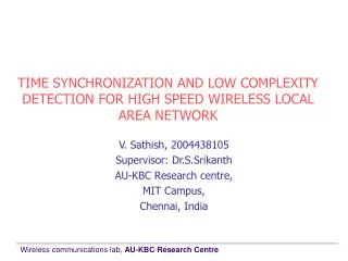
TIME SYNCHRONIZATION AND LOW COMPLEXITY DETECTION FOR HIGH SPEED WIRELESS LOCAL AREA NETWORK

1. TIME SYNCHRONIZATION AND LOW COMPLEXITY DETECTION FOR HIGH SPEED WIRELESS LOCAL AREA NETWORK V. Sathish, 2004438105 Supervisor: Dr.S.Srikanth AU-KBC Research centre, MIT Campus, Chennai, India

2. Timing synchronization in IEEE 802.11n systems

3. Presentation Outline • Abstract • IEEE 802.11n standard, goals and its challenges • Review of IEEE 802.11a preamble and its usage • 802.11n operating modes and frame formats • Timing synchronization • Literature survey • Proposed coarse timing estimation • Proposed fine timing estimation • Simulation setup and results discussion • Conclusion

4. Abstract • A low complexity timing synchronization method for the systems leased on the MIMO-OFDM1 based 802.11n standard is proposed • Two high throughput operating modes in IEEE 802.11n: • Mixed mode where 802.11a/g legacy systems and 802.11n based MIMO-OFDM systems shall co-exist • Greenfield mode where only 802.11n enabled MIMO-OFDM systems exists • For timing synchronization purposes, • Mixed mode : short training field (STF) and long training field (LTF) in preamble • Greenfield mode : Only short training field in preamble • Essentially, two time sync algorithms are needed for MIMO modes • Proposed algorithm uses only STF for timing synchronization and achieves same performance as LTF based algorithm • The STF structure is same on both the modes, so a single time sync algorithm can be implemented for all the high throughput modes. 1MIMO-OFDM Multiple input multiple output – Orthogonal frequency division multiplexing

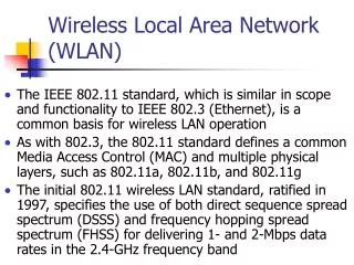
5. WLAN standards • Wi-Fi standards - IEEE 802.11 standard, 1997; 2 Mbps, 2.4GHz, CSMA/CA - IEEE 802.11b std, 1999; 11 Mbps, 2.4GHz, CSMA/CA - IEEE 802.11a std, 1999; 54 Mbps, 5GHz, CSMA/CA - IEEE 802.11g std, 2003; 11 Mbps & 54 Mbps, 2.4 GHz, CSMA/CA - IEEE 802.11n draft, 2006; 500 Mbps, 2.4 GHz, CSMA/CA

6. 802.11n standard Goals and its challenges • Achieve higher data rates (around 500 Mbps) • Use of MIMO-OFDM technology • Supports 20MHz and 40 MHz bandwidth operation • Interoperable with 802.11a/g legacy systems • Increased complexity • Multiple radio frequency (RF) and baseband (BB) chains required • Spatial detection techniques • Backward compatibility • MIMO-OFDM system should be able to decode the legacy packets • Legacy system should atleast know about the MIMO-OFDM transmission to avoid collision • Design of preamble impacts on initial receiver tasks

7. SIG GI SS Data SS SS LS1 LS2 Signal Field Short training field Long training field Review of IEEE802.11a frame Short symbols 1. Start of packet (SOP) detection 2. Automatic gain control (AGC) 3. Coarse timing estimation 4. Coarse frequency offset estimation Receiver tasks Long symbols 5. Fine timing estimation 6. Fine frequency offset estimation 7. Channel estimation 8. Data detection

8. Initial receiver tasks AGC & Synchro. Mode Acquisition mode Start of packet Packet detected End of packet Time & frequency Acquired Data detection Correction & Tracking mode Ch. Estimation Mode Offset update Channel estimated

9. SS SS SS LS CP LS SIG DATA Short training field Long training field 802.11n frame formats Non-High Throughput frame format • Used in the legacy network where only the 802.11a/g enabled devices are present • Content is identical to the frame defined in the IEEE 802.11a standard • STF – Short training field • LTF – Long training field

10. Legacy format Preamble High throughput Preamble HT-LTFn HT-SIG HT-STF L-STF L-LTF L-SIG HT-LTF 802.11n frame formats – contd. High throughput mixed frame format • High throughput stations and legacy stations shall co-exists • MIMO stations should transmit and receive the legacy frames and HT frames • For compatibility reasons, Initial preamble part is provided with the first three fields of non-HT preamble • HT-SIG, HT-STF and HT-LTFs are used decoding the MIMO packets • If the tranmission is intended for MIMO_OFDM system, then based on the number of TX antennas cyclic shift is applied as shown in table1 DATA

11. High throughput Preamble DATA HT-LTFn H-STF H-LTF H-SIG HT-LTF 802.11n frame formats – contd. High throughput Greenfield frame format • Only HT MIMO-OFDM stations can exist • All the training fields specific to MIMO-OFDM systems • HT-STF is identical to the L-STF field of mixed mode and is used for timing acquisition, AGC and frequency acquisition • For TH-SIG demodulation, channel estimates are obtained from first HT_LTF fields • Remaining HT-LTFs are used for estimating the channels across multiple transmit and receive antennas • Frames in different TX antennas are cyclically shifted based on table2 before transmission

12. Cyclic shift for HT frame transmission Table1. Cyclic shift for the non-HT portion of the packet Table2. Cyclic shift for the HT portion of the packet

13. 802.11n Access point For Backward compatibility Mixed mode Legacy mode • Preamble should be • compatible to legacy stations • Should work better for • MIMO-OFDM systems Only frames in legacy format Green field mode Preambles that are specific to MIMO-OFDM systems

14. 802.11n Access point 802.11n 802.11n 802.11n 802.11n 802.11g 802.11g 802.11g 802.11g Active node 802.11g Inactive node Typical 802.11n network Mixed mode Legacy mode Green field mode

15. Spatial Detection Spatial Demux Spatial Mux OFDM TX OFDM RX OFDM TX OFDM RX Transmitter Receiver channel Typical MIMO-OFDM system model NtxNr MIMO-OFDM system

16. Received signal at the receive antenna where is the transmitted signal from the TX antenna is the impulse response of the channel between the transmit and receive antenna transmit antennas and is given as The total power transmitted is normalized across the is the channel length and remains static across RX antenna with zero mean and variance is the AWGN at the is the normalized frequency offset Received signal model

17. Timing synchronization • Timing synchronization • To estimate the sampling time of the OFDM symbol • The start of OFDM symbol varies based on the strongest path of the fading channel • Non-optimal sampling causes ISI and ICI • Done in two steps • Coarse timing offset (CTO) estimation • Fine timing offset (FTO) estimation • Coarse timing offset estimation • Rough estimate is obtained • After start of packet detection and AGC, timing estimator is triggered • Fine timing offset estimation • Optimal starting of OFDM symbol is obtained

18. Literature survey • In [4], T. M. Schmidl and D.C. Cox had proposed a maximum likelihood (Ml) synchronization timing estimation method for a SISO-OFDM system. • An extension of this method for MIMO-OFDM system was proposed in [5] by A. N. Mody and G.L. Stuber, and in [6] by A. Van Zelst and Tim C. W. Schenk. • The drawback of these methods is that the preambles assumed in the papers are not the same as in the 802.11n standards. • In [7], Jianhua Liu and Jian Li presented a timing synchronization technique for a preamble that is similar to the one in the 802.11n standard. • However, the computational complexity of this method is high due to the cross correlation performed on the LTF for fine timing estimation.

19. Coarse timing offset estimation • The objective of the CTO estimator is to find the rough starting position of any of the short symbol • Typically 5-6 blocks of SS is taken for AGC operation • Coarse timing estimation can be performed only after AGC convergence. • An easy way is to find the end of the STF by using the autocorrelation property of the received signal.

20. Proposed Coarse timing offset estimation

21. Proposed coarse timing estimation technique Step1: • A metric is calculated from the instant k at which the AGC is converged • This metric is similar to the one in [7] and is given as where and is the value of the cross correlation between the signal and noise terms is the sum of noise energy and value of cross correlation between the signal and noise terms

22. The value of metric can take different values based on the index. with is the sum of the cross correlation of the signal and noise terms, and cross correlation between samples from STF and LTF. Since the fields STF and LTF are highly uncorrelated, the parameter decreases with thereby reduction in The metric will form the end of the plateau and could be noisy due to AWGN and multipath fading conditions To have a smooth plateau, the current metric is filtered through a weight filter and is given as Where is the weight factor given to previous value and is the weight applied to the current metric Proposed CTO estimator – contd..

23. Plot of metric1 Threshold based detection Reference for metric The falling end of plateau is noisy and getting a coarse timing estimates will be erroneous Metric Metric forms a Plateau - 2x2 system under the channel D with SNR=10dB

24. A new metric which is the average power of a difference signal over a window of samples is defined from the instant The value of metric depends on the instant For with the metric will be represented as and represents the averaged power of the STF and LTF respectively Proposed CTO estimator – contd. Step2: The metric is given as The total averaged power of the difference signal will increase as n increases. This is because of the contributions from LTF A smoothing operation is done on the metric by weighted averaging and is given as

25. Intersection point M2 Plot of CTO metrics Metric plotted for a 2x2 system under the channel D without noise

26. The metrics and can be used to get a reliable estimate of the CTO Steady increase in metric2 from and steady decrease in the value of metric1 from The instant should lie within the range [ , ] Let be the intersecting point then this instant will be chosen as the CTO estimate when the conditions given below are satisfied , , Where is the number of samples used to make sure that the estimate is not a false alarm due to noise Proposed CTO estimator – contd. The intersection point between these two metrics is estimated as the coarse time At low SNR, both the metrics will be noisy and fluctuating and this would result in wrong estimate There might more than one intersecting point due to fluctuations To avoid this a simple condition is proposed

27. Plot of metrics Reference for metric 1 Metric 1 2x2 MIMO-OFDM system; Channel model D; SNR=10dB Reference for metric 2 Metric 2

28. Proposed Fine timing offset estimation

29. Proposed fine timing estimator The objective of the fine timing offset estimator is to find the exact start of the OFDM symbol In multipath channel conditions this might not be possible because the strongest path could occur at non-zero delays In the proposed FTO estimator, we find an index in the starting of the 9th SS where the sum of channel impulse response energy is maximum between the receive antenna and transmit antenna This is achieved by using the correlation property of the STF and the advantages of the cyclic shift Achieved in two steps

30. The fine timing offset estimation algorithm is triggered from the index The received signal at each receive antenna is correlated with all the transmit signals Let be the received signal at the RX antenna after coarse frequency offset correction, Then, the cross correlation output between RX antenna and TX antenna is given as Proposed FTO estimator – contd. Step1: A simple cross correlation is performed between the received signal and the transmit signal Since the received signal at each receive antenna contains multiple versions of the transmit signal in cyclically shifted manner, the cross correlation between the received signal and the transmit signal will result in multiple peaks

31. Proposed FTO estimator – contd. Each peak corresponds to the total channel energy between transmit and receive antennas The position corresponding to the first peak of the first receive antenna output sequence is the fine timing estimate For example Let us assume the coarse timing estimate and all the channel impulse responses have the strongest path at zero delay For the 4x4 mixed mode system The cross correlation output between the first transmit antenna signal and the first receive antenna signal will have 4 peaks placed consecutively from Detecting the first peak is quite tricky due to multiple peaks that corresponds to different channel power between transmit and receive antennas To choose the first peak, we propose a simple technique

32. 0 1 2… 13, 14, 15 0 1 2… 13, 14, 15 0 1 2… 13, 14, 15 0 1 2… 13, 14, 15 Cross correlated output - Example For a 4x4 system Antenna3 Antenna1 Antenna2 Antenna4

33. With reference to the table1a for mixed mode, we propose the metrics , and for different antenna configurations as shown below Proposed FTO estimator – contd. Step2: The cyclic shift 50us, 100us, 150us and 200us applied at the transmit antenna corresponds to numerical shift 15, 14, 13 and 12 that is applied at the correlated output obtained from different transmit signals. The index corresponding to the maximum of absolute of the metric is determined as the fine timing offset.

34. Complexity analysis In case of the conventional LTF based FTO estimator, the complex cross correlation should be performed between 64 samples length long symbol and the received signal. In the proposed FTO estimator, the cross correlation is performed between 16 samples length short symbol and the received signal

35. Simulation and performance analysis

36. Performance of coarse timing estimator • Probability distribution of CTO estimate is plotted • Compared to the performance of threshold based technique • System model • 2x2, 3x3 and 4x4 antenna configuration • MIMO Channel model • TGn channel models • SNR = 8dB

37. Parameters of coarse timing estimator • For threshold based technique as in [7] • Mixed mode and green field mode • Threshold c2=0.6 and Q2=15 samples • For proposed technique • Mixed mode and green field mode • Threshold =0.45 and Q=8 samples • Smoothing filter weight = 0.5 for both the metrics

38. Estimation accuracy of the CTO estimator is [0, ] Probability of coarse timing offset estimate of conventional and the proposed technique. Probability of getting zero CTO is high for the algorithm proposed in threshold based technique Significant probability of the CTO obtained using this algorithm is going beyond the defined estimation accuracy In the proposed algorithm, estimates are more stable and lie within the estimation range

39. Comparison of probability of CTO estimates for different antenna configurations Probability of CTO estimates within the estimation accuracy As the number of antenna increases, the spatial diversity is leveraged resulting in a better performance for higher antenna configuration Proposed algorithm performs better at the lower SNR values as compared to the CTO estimation algorithm in [7]

40. Impact of channel models Probability of CTO estimates within the estimation accuracy for proposed algorithm in different channel models The maximum probability is achieved at 10dB SNR for a 2x2 system Motivation to use only the STF for the fine timing offset estimation

41. Performance of fine timing estimator • Probability distribution of fine timing estimate is plotted • Compared to the performance of simple cross correlation based technique using LTF • System model • 2x2, 3x3 and 4x4 antenna configurations • MIMO Channel model • TGn channel models

42. Comparison of probability of FTO estimates with LTF based FTO estimator The estimation accuracy is defined with the range [0, 3]. Computationally complex LTF based FTO LTF will have slightly better performance as compared to proposed technique Due to better noise averaging The probabilities of the FTO estimates within the estimation accuracy is plotted for the 3x3 and 4x4 systems of mixed mode.

43. Conclusion • A low complexity time synchronization algorithm is proposed • The proposed techniques performs better even at lower SNRs. • Using only STF, a single coarse and fine timing estimation technique will be used for both the high throughput modes • Same performance is achieved as LTF based timing synchronization • Thereby reducing total complexity of the system

44. References [1]. IEEE P802.11n™/D2.00, “Draft standard for Information Technology-Telecommunications and information exchange between systems-Local and metropolitan area networks-Specific requirements-“, Feb 2007 [2]. IEEE 802.11a standard, ISO/IEC 8802-11:1999/Amd 1:2000(E), http://standards.ieee.org/getieee802/download/802.11a-1999.pdf [3]. IEEE 802.11g standard, Further Higher-Speed Physical Layer Extension inthe2.4GHzBand, http://standards.ieee.org/getieee802/download /802. 11g-2003.pdf [4] T. M. Schmidl and D.C. Cox, “Robust Frequency and Timing Synchronization for OFDM”, IEEE Trans. on Communications, vol. 45, no. 12, pp. 1613-1621, Dec. 1997. [5]. A. N. Mody and G.L. Stuber, “Synchronization for MIMO-OFDM systems,” in Proc. IEEE Global Commun. Conf., vol. 1, pp.509-513, Nov.2001 [6] A. Van Zelst and Tim C. W. Schenk, “Implementation of MIMO-OFMD based Wireless LAN systems”, IEEE Trans. On Signal Proc. Vol. 52, No.2, pp. 483-494, Feb 2004 [7] Jianhua Liu and Jian Li, “A MIMO system with backward compatibility for OFDM based WLANs”, EURASIP journal on Applied signal processing. Pp. 696-706, May 2004 [8] IEEE P802.11 TGn channel models, May 10 2004,http://www.ece. ariz ona.edu/~yanli/files/11-03-0940-04-000n-tgn-channel-models.doc

45. Low Complexity MIMO-OFDM System for High Speed WLANs

46. Presentation Outline • Introduction • System model and channel model • MIMO-OFDM1 detection techniques • Proposed Group ordered MMSE V-BLAST2 detection • Simulation results • Conclusion 1MIMO-OFDM Multiple input multiple output – Orthogonal frequency division multiplexing 2MMSE V-BLAST Minimum mean square error – Vertical bell labs layered space time system

47. Spatial Detection Spatial Demux Spatial Mux OFDM TX OFDM RX OFDM TX OFDM RX Transmitter Receiver channel Introduction • MIMO-OFDM is a promising technique to increase data transmission rate in wireless frequency selective fading channels[1,2] • The key technique behind the MIMO-OFDM system is the spatial detection at the receiver

48. 1 1 FEC Encoder Spatial mapping 1 1 Interleaver Interleaver QAM Mapper QAM Mapper Encoder Parser Scrambler Stream Parser FEC Encoder IFFT & CP IFFT & CP 802.11n MIMO OFDM baseband transmitter 802.11n MIMO-OFDM baseband transmitter

49. 1 1 1 DECODER Stream De-parser Spatial Detector and demapping (Zero forcing, MMSE, SIC, etc) QAM De-Mapper QAM De-Mapper De interleaver De interleaver Descrambler M U X CP & FFT CP & FFT DECODER Decoded bits RX antennas 802.11n MIMO OFDM baseband receiver 802.11n MIMO-OFDM baseband receiver

50. Signal model and MIMO channel Received signal: After removing cyclic prefix and FFT operations, the received signal vector corresponding to subcarrier (bar over a variable represents vector) (1) where Transmit signal vector Additive white Gaussian Noise