WAVELETS AND FILTER BANKS
WAVELETS AND FILTER BANKS. Ildikó László, PhD ELTE UNIV., BUDAPEST, HUNGARY ildiko@inf.elte.hu. NEWER VERSION BUT STILL NEEDS IMPROOVMENTS AND CORRECTIONS !!!. BIBLIOGRAPHY: - G. Strang, T. Nguyen:Wavelets and Filter Banks, Wellesly-Cambridge Press


WAVELETS AND FILTER BANKS
E N D
Presentation Transcript
WAVELETS AND FILTER BANKS IldikóLászló, PhD ELTE UNIV., BUDAPEST, HUNGARY ildiko@inf.elte.hu
NEWER VERSION BUT STILL NEEDS IMPROOVMENTS AND CORRECTIONS!!!
BIBLIOGRAPHY: - G. Strang, T. Nguyen:Wavelets and Filter Banks, Wellesly-Cambridge Press - F. Schipp, W.R. Wade:Transforms on Normed Fields - Ingrid Daubechies: Ten Lectures on Wavelets - Stephane Mallat: A Wavelet tour of Signal Processing - Charles K. Chui: An Introduction to Wavelets etc.
AT THE END YOU WILL HAVE TO BE ABLE TO „GET” THINGS LIKE:
Some rows (10...) of A4: 50 100 150 200 250 50 100 150 200 250 50 100 150 200 250
Some rows (10...) of A3: 50 100 150 200 250 50 100 150 200 250 50 100 150 200 250
Some rows (22...) of A4: 50 100 150 200 250 50 100 150 200 250 50 100 150 200 250
Some rows (48...) of A3: 50 100 150 200 250 50 100 150 200 250 50 100 150 200 250
INTRODUCTION • - the classical Fourier analysis where a signal is • represented by its trigonometric Fourier • transform, is one of the most widely spread tools • in signal and image processing; • - at the end of the 19th century Du Bois-Reymond • constructed a continuous function with divergent • Fourier series; • - Hilbert: whether there exist any orthonormal • system for which the Fourier series with respect to • this system do not posses this singularity?
- Alfred Haar in 1909 constructed such an orthonormal system for which the Haar-Fourier series of continuous functions converge uniformly: - This was the first wavelet; (1910, Szeged, PhD)
The basic goal of Fourier series is to take a • signal – considered as a function of time • variable t, and decompose it into its various • frequency components; • -The basic building blocks are sin(nt) and cos(nt), • which vibrate at a frequency of n times per • interval. • - Consider the following function:
- This function has three components that vibrate at frequency 1 – the sin(t) part, at frequency 3 – the 2cos(3t) part, at frequency 50 – the 0.3sin(50t) part; • we can express a function f(t) in terms • of the basis functions, sine and cosine:
A trigonometric expansion is a sum of the • form: where the sum could be finite or infinite. • One disadvantage of Fourier series is that its • building blocks, sines and cosines, are periodic • waves that continueforever.
- In many appl., given a signal one is interested in its frequency component locally in time; (similar to music notation, which tells the player which notes –frequency inf. –to play at any given moment) - The standard Fourier transform, also gives the frequency content of
, .
- but inf. concerning time-localization of e.g., high frequency bursts cannot be read off easily from - time localization can be achieved by first windowing the signal f(t) 1 g(t) 0
- which is the windowed Fourier transform; - cuts off only a well-localized slice of -The wavelet transform provides a similar time-frequency description, with a few important differences;
Fourier transform: - represents the frequency comp. of a signal - doesn‘t offer localization in time Wavelet transform: - cuts up a signal into frequency components - studies each component with a resolution matched to its scale - offers localization in time
- A wavelet is a function of zero average: - which is dilated byj and translated by k; - j is the scaling parameter; - k is the translation coeff.; allows us to move the time localization centre; f is localized around k;
Wavelets - compactly supported small waves (don‘t extend from –infty to +infty) Each wavelet - is built up from the same „MOTHER“ wavelet by translation and dilation wjk(x) = 2j/2w(2jx - k)
- the wavelet transform of f at the scale j and position k is computed by correlating f with the wavelet: - have only recently been used – 1988 Ingrid Daubechies
Wavelets: - basis functions - linearly indep. functions; Fourier and Wavelet transforms: - representation of a signal f(t) by basis functions
- The Fourier transform of a complex, two dimensional function f(x,y) is given by: - where and are referred to as frequencies; - the inverse Fourier transform
- that is, f(x,y) is a linear combination of elementary functions, where the complex number is a weighting factor; – when dealing with linear systems – this can be used for decomposing a complicated input signal into more simple inputs; - that is, the response of the system can be calculated as the superposition of the responses given by the system to each of these “elementary” functions of the form:
- Examples; - Fourier transform theorems; - Linear Systems. Invariant Linear Systems; - Sampling theory;
Let us consider a rectangular lattice of samples of the function g(x,y) as defined: g_s(x,y)=comb(x/X) comb(y/Y) y x Y X
The sampled function g consists of an array of • functions, spaced at intervals of width X in the x • direction and Y in the y direction. • The area under each function is proportional to • the value of the g function at that particular point. • The spectrum G_s of g_s can be found by convolving • the transform of the comb function with the transform • of g.
f G(f , f ) y x y G(f , f ) x y f y f x f x 1/X 1/Y
1.2 1.0 -1 -1.2 1 1 0 0 1 -1 0 0 0 0 1 1 0 0 1 -1 1.2 1 T = X= -1 -1.2 2.2 0.2 -2.2 0.2 y = T * x = = 1.1 1.1 -1.1 -1.1 x = T^(-1) *y = Compressed, reconstructed; y(1)=y(3)=0
Convolution – example: n = 0, 1, 2 k = 0, 1, 2 n=0 x(2) x(1) x(0) y(0)=h(0)x(0) h(0) h(1) h(2) n=1 x(2) x(1) x(0) y(1)=h(0)x(1)+ h(0) h(1) h(2) h(1)x(0) n=2 x(2) x(1) x(0) h(0) h(1) h(2) y(2)=h(0)x(2)+h(1)x(1)+h(2)x(0)
FILTERS - A Filter – a linear time-invariant operator; - can be characterized by its impulse response function; - acts on an input vector x; the output y: is a convolution of x and the impulse response of the system;
- let us consider the input signal x(n) with the pure frequency - then the output in the time domain is: - where the last term can be recognized as: the Fourier transform of the impulse response of the system:
What is the connection between: WAVELETS, FILTERS and FILTER BANKS? - it is the High_Pass that leads to w(t) - the Low_Pass filter leads to a scaling function: - the scaling function in continuous time comes from an infinite repetition of the lowpass filter, with rescaling at each repetition; - the wavelet follows from by just one application of the highpass filter.
- averages come from the scaling functions; - details come from the wavelets. signal at level j (local averages) + =signal at level (j+1) details at level j (local differences)
LOW-PASS FILTER –or MOVING • AVERAGE To build up the simplest lowpass filter, we use the Haar filter coefficients: h(0)=1/2 and h(1)=1/2. - the output at time t=n is the average of the input x(n) and that at time t=n-1 : x(n-1).
averaging filter=1/2 (identity) + 1/2 (delay) y(n)=1/2 x(n)+1/2 x(n-1) Every linear operator acting on a signal x can be represented by a matrix: y=H*x . x(-1) x(0) x(1) . . y(-1) y(0) y(1) . ½ 0 0 0 0 ½ ½ 0 0 0 0 ½ ½ 0 0 0 0 ½ ½ 0 0 0 0 . . =
- with the simple input signal, with pure frequency: - that is, the output can be written as: y(n)=SOMETHING * x(n) - this “something” is expressing the effect of our filter, or system on the input signal;
- The frequency response or transfer function of the system: - because this is a periodic function, we want: - it results: