
Homework
E N D
Presentation Transcript
Homework • Chapter 11: 13 • Chapter 12: 1, 2, 14, 16
The wrong way to make a comparison of two groups “Group 1 is significantly different from a constant, but Group 2 is not. Therefore Group 1 and Group 2 are different from each other.”
Interpreting Confidence Intervals Not different Unknown Different
Assumptions • Random sample(s) • Populations are normally distributed • Populations have equal variances • 2-sample t only
Assumptions • Random sample(s) • Populations are normally distributed • Populations have equal variances • 2-sample t only What do we do when these are violated?
Assumptions in Statistics • Are any of the assumptions violated? • If so, what are we going to do about it?
Detecting deviations from normality • Histograms • Quantile plots • Shapiro-Wilk test
Detecting deviations from normality: by histogram Frequency Biomass ratio
Detecting deviations from normality: by quantile plot Normal Quantile Normal data
Detecting deviations from normality: by quantile plot Normal Quantile Biomass ratio
Detecting deviations from normality: by quantile plot Normal Quantile Normal distribution = straight line Non-normal = non-straight line Biomass ratio
Detecting differences from normality: Shapiro-Wilk test Shapiro-Wilk Test is used to test statistically whether a set of data comes from a normal distribition Ho: The data come from a normal distribution Ha: The data come from some other distribution
What to do when the distribution is not normal • If the sample sizes are large, sometimes the standard tests work OK anyway • Transformations • Non-parametric tests • Randomization and resampling
The normal approximation • Means of large samples are normally distributed • So, the parametric tests on large samples work relatively well, even for non-normal data. • Rule of thumb- if n > ~50, the normal approximations may work
Data transformations A data transformation changes each data point by some simple mathematical formula
Log-transformation ln = “natural log”, base e log = “log”, base 10 EITHER WORK Y Y' = ln[Y]
Variance and mean increase together --> try the log-transform
Other transformations Arcsine Square-root Square Reciprocal Antilog
Example: Confidence interval with log-transformed data Data: 5 12 1024 12398 ln data: 1.61 2.48 6.93 9.43 ln[Y] ln[Y] ln[Y]
Valid transformations... • Require the same transformation be applied to each individual • Must be backwards convertible to the original value, without ambiguity • Have one-to-one correspondence to original values X = ln[Y] Y = eX
Choosing transformations • Must transform each individual in the same way • You CAN try different transformations until you find one that makes the data fit the assumptions • You CANNOT keep trying transformations until P <0.05!!!
Assumptions • Random sample(s) • Populations are normally distributed • Populations have equal variances • 2-sample t only Do the populations have equal variances? If so, what should We do about it?
Comparing the variance of two groups One possible method: the F test
The test statistic F Put the larger s2 on top in the numerator.
F... • F has two different degrees of freedom, one for the numerator and one for the denominator. (Both are df = ni -1.) The numerator df is listed first, then the denominator df. • The F test is very sensitive to its assumption that both distributions are normal.
Degrees of freedom For a 2-tailed test, we compare to Fa/2,df1,df2 from Table A3.4
Why a/2 for the critical value? By putting the larger s2 in the numerator, we are forcing F to be greater than 1. By the null hypothesis there is a 50:50 chance of either s2 being greater, so we want the higher tail to include just a/2.
Conclusion The F= 107.4 from the data is greater than F(0.025), 6,8 =4.7, so we can reject the null hypothesis that the variances of the two groups are equal. The variance in insect genitalia is much greater for polygamous species than monogamous species.
F-test Null hypothesis The two populations have the same variance 21 22 Sample Null distribution F with n1-1, n2-1 df Test statistic compare How unusual is this test statistic? P > 0.05 P < 0.05 Reject Ho Fail to reject Ho
What if we have unequal variances? • Welch’s t-test would work • If sample sizes are equal and large, then even a ten-fold difference in variance is approximately OK
Comparing means when variances are not equal Welch’s t test compared the means of two normally distributed populations that have unequal variances
Experimental design • 20 randomly chosen burrowing owl nests • Randomly divided into two groups of 10 nests • One group was given extra dung; the other not • Measured the number of dung beetles on the owls’ diets
Number of beetles caught • Dung added: • No dung added:
Hypotheses H0: Owls catch the same number of dung beetles with or without extra dung (m1 = m2) HA: Owls do not catch the same number of dung beetles with or without extra dung (m1m2)
Welch’s t Round down df to nearest integer
Degrees of freedom Which we round down to df= 10
Reaching a conclusion t0.05(2), 10= 2.23 t=4.01 > 2.23 So we can reject the null hypothesis with P<0.05. Extra dung near burrowing owl nests increases the number of dung beetles eaten.
Assumptions • Random sample(s) • Populations are normally distributed • Populations have equal variances • 2-sample t only What if you don’t want to make so many assumptions?
Welch’s t-test Null hypothesis The two populations have the same mean 12 Sample Null distribution t with df from formula Test statistic compare How unusual is this test statistic? P > 0.05 P < 0.05 Reject Ho Fail to reject Ho
Non-parametric methods • Assume less about the underlying distributions • Also called "distribution-free" • "Parametric" methods assume a distribution or a parameter