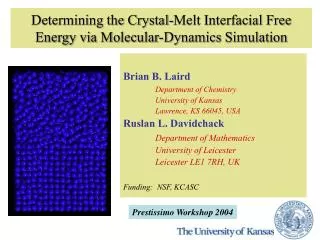
Determining the Crystal-Melt Interfacial Free Energy via Molecular-Dynamics Simulation

1. Determining the Crystal-Melt Interfacial Free Energy via Molecular-Dynamics Simulation Brian B. Laird Department of Chemistry University of Kansas Lawrence, KS 66045, USA Ruslan L. Davidchack Department of Mathematics University of Leicester Leicester LE1 7RH, UK Funding: NSF, KCASC Prestissimo Workshop 2004

2. Observation #1 Not all important problems addressed with MD simulation are biological. In this work we describe application of molecular simulation to an important problem in materials science/metallurgy Material Properties Molecular Interactions

3. Solid Liquid Problem: Can one calculate the free energy of a crystal-melt interface using MD simulation? Crystal-melt interfacial free energy, gcl • The work required to form a unit area of interface between a crystal and its own melt

4. Why is the Interfacial Free Energy Important? cl is a primary controlling parameter governing the kinetics and morphology of crystal growth from the melt Experiment Model Example:Dendritic Growth The nature of dendritic growth from the melt is highly sensitive to the orientation dependence (anisotropy) in cl. Data from simulation can be used in continuum models of dendrite growth kinetics (Phase-field modeling) Growth of dendrites in succinonitrile (NASA microgravity program)

5. Why is the Interfacial Free Energy Important? cl is a primary controlling parameter governing the kinetics and morphology of crystal growth from the melt Observation of nucleation in colloidal crystals: Weitz group (Harvard) Example:Crystal nucleation The rate of homogeneous crystal nucleation from under-cooled melts is highly dependent on the magnitude of cl Nucleation often occurs not to the thermodynamically most stable bulk crystal phase, but to the one with the lowest kinetic barrier (i.e. lowest cl) - Ostwald step rule

6. Why are simulations necessary here? Direct experimental determination of gclis difficult and few measurements exist • Direct measurements: (contact angle) • Only a handful of materials: water, cadmium, bismuth, pivalic acid, succinonitrile • Indirect measurements: (nucleation) • Primary source of data for g. Accurate only to 10-20% Simulations needed to determine phenomenology

7. Indirect experimental measurement of gcl(Nucleation data and Turnbull’s rule) gcl can be estimated from nucleation rates: typically accurate to 10-20% Turnbull (1950) estimated gcl from nucleation rate data and found the following empirical rule: gcl r-2/3 =CT DfusH where the Turnbull Coefficient CTis ~.45 for metals and ~ 0.32 for non-metals Can we understand the molecular origin of Turnbull’s Rule???

8. Calculating Free Energies via simulation:Why is Free Energy hard to measure? • Unlike energy, entropy (& free Energy) is not the average of some mechanical variable, but is a function of the entire trajectory (or phase space) • Free energy, F = E - TS, calculation generally require a series of simulations slowly transforming the system from a reference state to the state of interest Thermodynamic Integration Frenkel Analogy Energy  Depth of lake Entropy  Volume of Lake

9. Observation #2 In molecular simulation there are almost always two (or more) very different methods for calculating any given quantity Calculating a quantity of interest using more than one method is an important check on the efficacy of our methods Cleaving Method gcl Fluctuation Method

10. Fluctuation Method • Method due to Hoyt, Asta & Karma, PRL 86 5530, (2000) • h(x) = height of an interface in a quasi two-dimensional slab • If q= angle between the average interface normal and its instantaneous value, then the stiffness of the interface can be defined • The stiffness can be found from the fluctuations in h(x) • Advantage: • Anisotropy in g precisely measured • Disadvantages: • Large systems (N = 40,000 - 100,000) • Low precision in g itself h(x) W b

11. Cleaving methods for calculating interfacial free energy • Cleaving Potentials: Broughton & Gilmer (1986) - Lennard-Jones system • Cleaving Walls: Davidchack & Laird (2000) - HS, LJ, Inverse-Power potentials • Advantages:very precise for g, relatively small sizes (N = 7000 - 10,000) • Disadvantages: Anisotropy measurement not as precise as in fluctuation method Calculate g directly by cleaving and rearrang-ing bulk phases to give interface of interest THERMODYNAMIC INTEGRATION crystal cry stal + liquid liq uid + cry uid cry uid

12. How is the cleaving done? • Choose a dividing surface – particles to the left of the surface are labeled “1”, those to the right are labeled “2” • Wall labeled “1” interacts only with particles of type “1”, same for “2” • As walls “1” and “2” are moved in opposite directions toward one another the two halves of the system are separated • If separation done slowly enough the cleaving is reversible • Work/Area to cleave measured be integrating the pressure on the walls as a function of wall position. We employ special cleaving walls made of particles similar to those in the system

13. Observation #3 Physical reality is overrated in molecular simulation In calculating free energies via simulation, we only care that the initial and final states are “physical”, we can do (almost) anything we want in between

14. Solid Liquid Start with separate solid and liquid systems equilibrated at coexistence conditions: T, rc, rf Step 1 Step 2 Steps 1, 2: Insert suitably chosen “cleaving” potentials into the solid and liquid systems A B B A Step 3 Step 3: Juxtapose the solid and liquid systems by rearranging the boundary conditions while maintaining the cleaving potentials A A B B Step 4 Step 4: Remove the cleaving potentials from the combined system gA = w1 + w4 + w3 + w4 Cleaving methods for calculating interfacial free energy

15. Systematic error: hysteresis The main source of uncertainty in the obtained results is the presence of a hysteresis loop at the fluid ordering transition in Step 2 • Reducing Hysteresis • longer runs • improve cleaving wall design • cleave fluid at lower density (adds an extra step)

16. Our approach: a systematic study of the effect of inter-atomic potential on cl • Simplest potential - Hard spheres • Effect of Attraction - Lennard Jones • Effect of range of repulsive potential - inverse power potentials

17. First Study: The Simplest SystemHard Spheres Why hard spheres? Hard Sphere Model Typical Simple Material The freezing transition of simple liquids can be well described using a hard-sphere model

18. The Hard-Sphere Crystal Face-Centered Cubic (FCC)

19. Simulation Details for Hard-Spheres • Hard-sphere MD algorithmically exact: Chain of exactly resolved elastic collisions • Rappaport’s cell method: dramatically speeds up collision detection • (100), (110) and (111) interfaces studied • N ~ 10,000 particles • Phase coexistence independent of T: rs3 = 1.037 (crystal); 0.939 (fluid) • g = g1kBT/s 2

20. Results for hard-spheres[Davidchack & Laird, PRL 85 4751 (2000)] g[100] = 0.592(7) kT/s2 g[110] = 0.571(6) kT/s2 g[111] = 0.557(7) kT/s2 • How do these numbers fit in with other estimates? • From Nucleation Experiments on silica microspheres • 0.54 to 0.55kT/s2 (Marr&Gast 94, Palberg 99) • From Density-Functional Theory: • predictions range from 0.28 - 2.00 kT/s2 • (WDA of Curtin & Ashcroft gives 0.62 kT/s2) • From Simulation: Frenkel nucleation simulations: 0.61 kT/s2

21. Can Turnbull’s rule be explained with a hard-sphere model? For hard-spheres, Turnbull’s reduced interfacial free energy scales linearly with the melting temperature • = 0.57 (0.55) kTm/s2 g rs-2/3 = 0.55(0.53)Tmsince rs = 1.037 s-3 If a hard-sphere model holds one would predict that g rs-2/3= C Tm with C ~ 0.5-0.6

22. Hard-Sphere Model for FCC forming metals g rs-2/3 ~ 0.5 kTm Turnbull’s rule follows since DfusS = DfusH/Tm is nearly constant for these metals

23. Continuous Potentials • Lennard-Jones • Inverse-Power Potentials Differences with Hard-spheres • w3 is non-zero • More care must be taken in construction of cleaving wall potential • need to use NVT simulation to maintain coexistence temperature throughout simulation (e.g., use Nose´-Hoover or Nose´-Poincare methods)

24. Observation #4 In precise simulation work it is important to always be aware of the damage done to statistical mechanical averages by the discretization Free energy simulations involving phase equilibrium require highly precise simulations and discretization error in averages can be important Need: a detailed statistical mechanics of numerical algorithms

25. Example of the effect of discretization errorin Nose´-Poincare´ MD • In Nose´NVT dynamics, constant T is maintained by adding two new variables to the Hamiltonian • In Nose´-Poincare´ (Bond, Leimkuhler & Laird, 1999) the Nose´ Hamiltonian is time transformed to run in real time • Can be integrated using the Generalized Leapfrog Algorithm (GLA) • GLA is symplectic • g = Number of degrees of freedom • NVE dynamics generated by HN , after time transformation dt/dt=s, yields a canonical (NVT) distribution in the reduced phase space

26. Example of the effect of discretization errorin Nose´-Poincare´ MD • If canonical distribution is correctly obtained then the equipartition theorem holds • The difference between T and Tinst is a measure of the uncertainty in T due to the discretization • For Nose´-Poincare´ with GLA this can be worked out (S. Bond thesis). Similar formulae for Nose´-Hoover integrators

27. Results for the truncated Lennard-Jones system(Davidchack & Laird, J. Chem. Phys., 118, 7651 (2003) *J.Chem.Phys. 84, 5759 (1986). Note that anisotropy in LJ differs from HS in that the order of (110) and (111) are switched.

28. ANISOTROPY in Interfacial Free Energy Expansion in cubic harmonics (Fehlner & Vosko)

29. Inverse Power Potentials • Important reference system for studying the effect of potential range • For n=∞, we have the hard-sphere system. • Phase Diagram: For n>7, crystal structure is FCC, for 4<n<7 system freezes to BCC transforming to FCC at lower temperatures (higher densities) fluid fcc n > 7 density fluid bcc fcc n < 7

30. Inverse Power Potential Scaling • Only one parameter esn • Excess thermodynamic properties only depend upon • Gn = rs3 (kT/e)-3/n = r* T*-3/n • Phase diagram is one dimensional, only depends upon Gn • Along coexistence curve: • Pc = P1T(1+3/n); g = g1 T(1 + 2/n)

31. Inverse Power Potentials and Turnbull’s rule From the scaling laws So… as in hard spheres, we see scaling with Tm Turnbull’s rule is exact for inverse power potentials! And since DHfus = TDSfus

32. Results for the Inverse-Power Series Similar to Fe (Asta, et al.) the bcc interface has a lower free energy

33. Turnbull Coefficient Similar to Fe (Asta, et al.) the bcc interface has a lower free energy

34. Results for the Inverse-Power Series(Anisotropy) Similar to Fe (Asta, et al.) the bcc interface has a anisotropy

35. Summary • We have measured the crystal/melt interfacial free energy, g, for hard-spheres, Lennard-Jones and inverse-power series. Our simulations can resolve the anisotropy in this quantity. • Comparison of data from fluctuation method and cleaving method shows the two methods to be consistent and complementary • We show the molecular origin of Turnbull’s rule and give an alternate formulation • For the inverse-power series gbcc < gfcc consistent with fluctuation model calculations and nucleation experiments - also bcc is less anisotropic than fcc.